Machine learning is an expansive field – one often made better by techniques common to data science like regression.
In this tutorial, we’re going to explore the topic of neural networks and discover how we can make use of regression techniques when working with them. We’ll also dive into how to use Python to work with these concepts.
Let’s dive in and start learning!
Intro to Neural Networks and RBF Nets
Neural Networks are very powerful models for classification tasks. But what about regression? Suppose we had a set of data points and wanted to project that trend into the future to make predictions. Regression has many applications in finance, physics, biology, and many other fields.
Radial Basis Function Networks (RBF nets) are used for exactly this scenario: regression or function approximation. We have some data that represents an underlying trend or function and want to model it. RBF nets can learn to approximate the underlying trend using many Gaussians/bell curves.
Prerequisites
You can download the full code here.
Before we begin, please familiarize yourself with neural networks, backpropagation, and k-means clustering. Alternatively, if this is your first foray into the world of machine learning, we recommend first learning the fundamentals of Python. You can check out our tutorials, or try a robust curriculum like the Python Mini-Degree to do so.
For educators, we can also recommend Zenva Schools. Not only does the platform have tons of online courses for Python, but is suitable for K12 environments with classroom management tools, course plans, and more.

BUILD YOUR OWN GAMES
Get 250+ coding courses for
$1
AVAILABLE FOR A LIMITED TIME ONLY
RBF Nets
An RBF net is similar to a 2-layer network. We have an input that is fully connected to a hidden layer. Then, we take the output of the hidden layer perform a weighted sum to get our output.
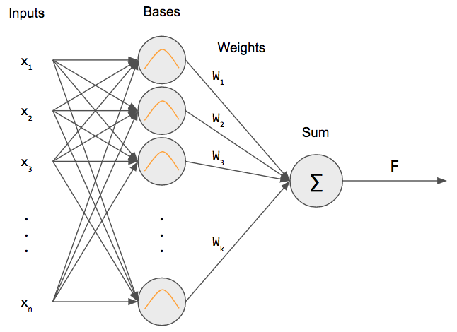
But what is that inside the hidden layer neurons? That is a Gaussian RBF! This differentiates an RBF net from a regular neural network: we’re using an RBF as our “activation” function (more specifically, a Gaussian RBF).
Gaussian Distribution
The first question you may have is “what is a Gaussian?” It’s the most famous and important of all statistical distributions. A picture is worth a thousand words so here’s an example of a Gaussian centered at 0 with a standard deviation of 1.
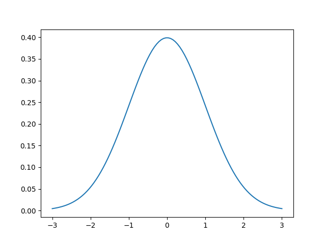
This is the Gaussian or normal distribution! It is also called a bell curve sometimes. The function that describes the normal distribution is the following
\[ \mathcal{N}(x; \mu, \sigma^2) = \displaystyle\frac{1}{\sqrt{2\pi\sigma^2}}e^{-\displaystyle\frac{(x-\mu)^2}{2\sigma^2}} \]
That looks like a really messy equation! And it is, so we’ll use $\mathcal{N}(x; \mu, \sigma^2)$ to represent that equation. If we look at it, we notice there are one input and two parameters. First, let’s discuss the parameters and how they change the Gaussian. Then we can discuss what the input means.
The two parameters are called the mean $\mu$ and standard deviation $\sigma$. In some cases, the standard deviation is replaced with the variance $\sigma^2$, which is just the square of the standard deviation. The mean of the Gaussian simply shifts the center of the Gaussian, i.e. the “bump” or top of the bell. In the image above, $\mu=0$, so the largest value is at $x=0$.
The standard deviation is a measure of the spread of the Gaussian. It affects the “wideness” of the bell. Using a larger standard deviation means that the data are more spread out, rather than closer to the mean.
Technically, the above function is called the probability density function (pdf) and it tells us the probability of observing an input $x$, given that specific normal distribution. But we’re only interested in the bell-curve properties of the Gaussian, not the fact that it represents a probability distribution.
Gaussians in RBF nets
Why do we care about Gaussians? We can use a linear combination of Gaussians to approximate any function!
Source: https://terpconnect.umd.edu/~toh/spectrum/CurveFittingB.html
In the figure above, the Gaussians have different colors and are weighted differently. When we take the sum, we get a continuous function! To do this, we need to know where to place the Gaussian centers $c_j$ and their standard deviations $\sigma_j$.
We can use k-means clustering on our input data to figure out where to place the Gaussians. The reasoning behind this is that we want our Gaussians to “span” the largest clusters of data since they have that bell-curve shape.
The next step is figuring out what the standard deviations should be. There are two approaches we can take: set the standard deviation to be that of the points assigned to a particular cluster $c_j$ or we can use a single standard deviation for all clusters $\sigma_j = \sigma \forall j$ where $\sigma=\frac{d_\text{max}}{\sqrt{2k}}$ where $d_\text{max}$ is the maximum distance between any two cluster centers. and $k$ is the number of cluster centers.
But wait, how many Gaussians do we use? Well that’s a hyperparameter called the number of bases or kernels $k$.
Backpropagation for RBF nets
K-means clustering is used to determine the centers $c_j$ for each of the radial basis functions $\varphi_j$. Given an input $x$, an RBF network produces a weighted sum output.
\begin{equation*}
F(x)=\displaystyle\sum_{j=1}^k w_j\varphi_j(x, c_j) + b
\end{equation*}
where $w_j$ are the weights, $b$ is the bias, $k$ is the number of bases/clusters/centers, and $\varphi_j(\cdot)$ is the Gaussian RBF:
\begin{equation*}
\varphi_j(x, c_j) = \exp\left(\displaystyle\frac{-||x-c_j||^2}{2\sigma_j^2} \right)
\end{equation*}
There are other kinds of RBFs, but we’ll stick with our Gaussian RBF. (Notice that we don’t have the constant up front, so our Gaussian is not normalized, but that’s ok since we’re not using it as a probability distribution!)
Using these definitions, we can derive the update rules for $w_j$ and $b$ for gradient descent. We use the quadratic cost function to minimize.
\begin{equation*}
C = \displaystyle\sum_{i=1}^N (y^{(i)}-F(x^{(i)}))^2
\end{equation*}
We can derive the update rule for $w_j$ by computing the partial derivative of the cost function with respect to all of the $w_j$.
\begin{align*}
\displaystyle\frac{\partial C}{\partial w_j} &= \displaystyle\frac{\partial C}{\partial F} \displaystyle\frac{\partial F}{\partial w_j}\\
&=\displaystyle\frac{\partial }{\partial F}[\displaystyle\sum_{i=1}^N (y^{(i)}-F(x^{(i)}))^2]~\cdot~\displaystyle\frac{\partial }{\partial w_j}[\displaystyle\sum_{j=0}^K w_j\varphi_j(x,c_j) + b]\\
&=-(y^{(i)}-F(x^{(i)}))~\cdot~\varphi_j(x,c_j)\\
w_j &\gets w_j + \eta~(y^{(i)}-F(x^{(i)}))~\varphi_j(x,c_j)
\end{align*}
Similarly, we can derive the update rules for $b$ by computing the partial derivative of the cost function with respect to $b$.
\begin{align*}
\displaystyle\frac{\partial C}{\partial b} &= \displaystyle\frac{\partial C}{\partial F} \displaystyle\frac{\partial F}{\partial b}\\
&=\displaystyle\frac{\partial }{\partial F}[\displaystyle\sum_{i=1}^N (y^{(i)}-F(x^{(i)}))^2]~\cdot~\displaystyle\frac{\partial }{\partial b}[\displaystyle\sum_{j=0}^K w_j\varphi_j(x,c_j) + b]\\
&=-(y^{(i)}-F(x^{(i)}))\cdot 1\\
b &\gets b + \eta~(y^{(i)}-F(x^{(i)}))
\end{align*}
Now we have our backpropagation rules!
RBF Net Code
Now that we have a better understanding of how we can use neural networks for function approximation, let’s write some code!
First, we have to define our “training” data and RBF. We’re going to code up our Gaussian RBF.
def rbf(x, c, s):
    return np.exp(-1 / (2 * s**2) * (x-c)**2)
Now we’ll need to use the k-means clustering algorithm to determine the cluster centers. I’ve already coded up a function for you that gives us the cluster centers and the standard deviations of the clusters.
def kmeans(X, k):
    """Performs k-means clustering for 1D input

    Arguments:
        X {ndarray} -- A Mx1 array of inputs
        k {int} -- Number of clusters

    Returns:
        ndarray -- A kx1 array of final cluster centers
    """

    # randomly select initial clusters from input data
    clusters = np.random.choice(np.squeeze(X), size=k)
    prevClusters = clusters.copy()
    stds = np.zeros(k)
    converged = False

    while not converged:
        """
        compute distances for each cluster center to each point
        where (distances[i, j] represents the distance between the ith point and jth cluster)
        """
        distances = np.squeeze(np.abs(X[:, np.newaxis] - clusters[np.newaxis, :]))

        # find the cluster that's closest to each point
        closestCluster = np.argmin(distances, axis=1)

        # update clusters by taking the mean of all of the points assigned to that cluster
        for i in range(k):
            pointsForCluster = X[closestCluster == i]
            if len(pointsForCluster) > 0:
                clusters[i] = np.mean(pointsForCluster, axis=0)

        # converge if clusters haven't moved
        converged = np.linalg.norm(clusters - prevClusters) < 1e-6
        prevClusters = clusters.copy()

    distances = np.squeeze(np.abs(X[:, np.newaxis] - clusters[np.newaxis, :]))
    closestCluster = np.argmin(distances, axis=1)

    clustersWithNoPoints = []
    for i in range(k):
        pointsForCluster = X[closestCluster == i]
        if len(pointsForCluster) < 2:
            # keep track of clusters with no points or 1 point
            clustersWithNoPoints.append(i)
            continue
        else:
            stds[i] = np.std(X[closestCluster == i])

    # if there are clusters with 0 or 1 points, take the mean std of the other clusters
    if len(clustersWithNoPoints) > 0:
        pointsToAverage = []
        for i in range(k):
            if i not in clustersWithNoPoints:
                pointsToAverage.append(X[closestCluster == i])
        pointsToAverage = np.concatenate(pointsToAverage).ravel()
        stds[clustersWithNoPoints] = np.mean(np.std(pointsToAverage))

    return clusters, stds
This code just implements the k-means clustering algorithm and computes the standard deviations. If there is a cluster with none or one assigned points to it, we simply average the standard deviation of the other clusters. (We can’t compute standard deviation with no data points, and the standard deviation of a single data point is 0).
We’re not going to spend too much time on k-means clustering. Visit the link at the top for more information.
Now we can get to the real heart of the RBF net by creating a class.
class RBFNet(object):
    """Implementation of a Radial Basis Function Network"""
    def __init__(self, k=2, lr=0.01, epochs=100, rbf=rbf, inferStds=True):
        self.k = k
        self.lr = lr
        self.epochs = epochs
        self.rbf = rbf
        self.inferStds = inferStds

        self.w = np.random.randn(k)
        self.b = np.random.randn(1)
We have options for the number of bases, learning rate, number of epochs, which RBF to use, and if we want to use the standard deviations from k-means. We also initialize the weights and bias. Remember that an RBF net is a modified 2-layer network, so there’s only only one weight vector and a single bias at the output node, since we’re approximating a 1D function (specifically, one output). If we had a function with multiple outputs (a function with a vector-valued output), we’d use multiple output neurons and our weights would be a matrix and our bias a vector.
Then, we have to write our fit function to compute our weights and biases. In the first few lines, we either use the standard deviations from the modified k-means algorithm, or we force all bases to use the same standard deviation computed from the formula. The rest is similar to backpropagation where we propagate our input going forward and update our weights going backward.
def fit(self, X, y):
    if self.inferStds:
        # compute stds from data
        self.centers, self.stds = kmeans(X, self.k)
    else:
        # use a fixed std
        self.centers, _ = kmeans(X, self.k)
        dMax = max([np.abs(c1 - c2) for c1 in self.centers for c2 in self.centers])
        self.stds = np.repeat(dMax / np.sqrt(2*self.k), self.k)

    # training
    for epoch in range(self.epochs):
        for i in range(X.shape[0]):
            # forward pass
            a = np.array([self.rbf(X[i], c, s) for c, s, in zip(self.centers, self.stds)])
            F = a.T.dot(self.w) + self.b

            loss = (y[i] - F).flatten() ** 2
            print('Loss: {0:.2f}'.format(loss[0]))

            # backward pass
            error = -(y[i] - F).flatten()

            # online update
            self.w = self.w - self.lr * a * error
            self.b = self.b - self.lr * error
For verbosity, we’re printing the loss at each step. Notice we’re also performing an online update, meaning we update our weights and biases each input. Alternatively, we could have done a batch update, where we update our parameters after seeing all training data, or minibatch update, where we update our parameters after seeing a subset of the training data.
Making a prediction is as simple as propagating our input forward.
def predict(self, X):
    y_pred = []
    for i in range(X.shape[0]):
        a = np.array([self.rbf(X[i], c, s) for c, s, in zip(self.centers, self.stds)])
        F = a.T.dot(self.w) + self.b
        y_pred.append(F)
    return np.array(y_pred)
Notice that we’re allowing for a matrix inputs, where each row is an example.
Finally, we can write code to use our new class. For our training data, we’ll be generating 100 samples from the sine function. Then, we’ll add some uniform noise to our data.
# sample inputs and add noise
NUM_SAMPLES = 100
X = np.random.uniform(0., 1., NUM_SAMPLES)
X = np.sort(X, axis=0)
noise = np.random.uniform(-0.1, 0.1, NUM_SAMPLES)
y = np.sin(2 * np.pi * X)  + noise

rbfnet = RBFNet(lr=1e-2, k=2)
rbfnet.fit(X, y)

y_pred = rbfnet.predict(X)

plt.plot(X, y, '-o', label='true')
plt.plot(X, y_pred, '-o', label='RBF-Net')
plt.legend()

plt.tight_layout()
plt.show()
We can plot our approximated function against our real function to see how well our RBF net performed.
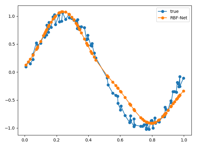
From our results, our RBF net performed pretty well! If we wanted to evaluate our RBF net more rigorously, we could sample more points from the same function, pass it through our RBF net and use the summed Euclidean distance as a metric.
We can try messing around with some key parameters, like the number of bases. What if we increase the number of bases to 4?
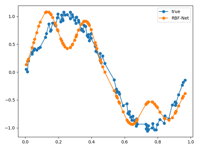
Our results aren’t too great! This is because our original function is shaped the way that it is, i.e., two bumps. If we had a more complicated function, then we could use a larger number of bases. If we used a large number of bases, then we’ll start overfitting!
Another parameter we can change is the standard deviation. How about we use a single standard deviation for all of our bases instead of each one getting its own?
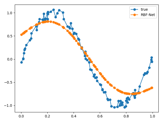
Our plot is much smoother! This is because the Gaussians that make up our reconstruction all have the same standard deviation.
There are other parameters we can change like the learning rate; we could use a more advanced optimization algorithm; we could try layering Gaussians; etc.
To summarize, RBF nets are a special type of neural network used for regression. They are similar to 2-layer networks, but we replace the activation function with a radial basis function, specifically a Gaussian radial basis function. We take each input vector and feed it into each basis. Then, we do a simple weighted sum to get our approximated function value at the end. We train these using backpropagation like any neural network! Finally, we implemented RBF nets in a class and used it to approximate a simple function.
RBF nets are a great example of neural models being used for regression!
Want to learn more about how Python can help your career? Check out this article! You can also expand your Python skills with the Python Mini-Degree or, for teachers in need of classroom resources, the Zenva Schools platform.
BUILD GAMES

FINAL DAYS: Unlock 250+ coding courses, guided learning paths, help from expert mentors, and more.

