Introduction to Convolutional Neural Networks for Vision Tasks

Neural networks have been used for a wide variety of tasks across different fields. But what about image-based tasks? We’d like to do everything we could with a regular neural network, but we want to explicitly treat the inputs as images. We’ll discuss a special kind of neural network called a Convolutional Neural Network (CNN) that lies at the intersection between Computer Vision and Neural Networks. CNNs are used for a wide range of image-related tasks such as image classification, object detection/localization, image generation, visual question answering, and more! We’ll discuss the different kinds of layers in a CNN and how they function. Finally, we will build a historical CNN architecture called LeNet-5 and use it to recognize handwritten digits using the Keras library (on top of Tensorflow). Download the full code here.

If you’re not familiar with neural networks or the MNIST dataset, I highly recommend acquainting yourself by reading the post here. You’ll also need to install Tensorflow and Keras for your system.

Table of contents

Convolutional Neural Networks Overview

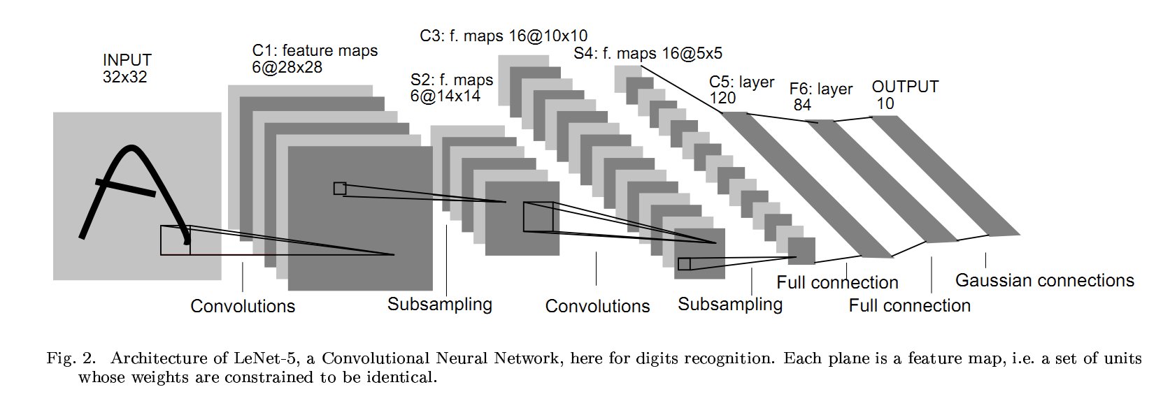
Let’s look at the CNN we’ll be constructing: LeNet-5.

(Gradient-Based Learning Applied to Document Recognition by LeCun et al.)

From this architecture, we notice is that the input is the full image itself. We don’t flatten it in any way! This is good because we’re maintaining the spatial relations between pixels. When we flatten it, we lose that spatial information.

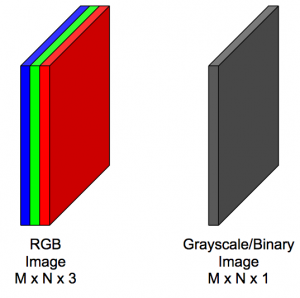
Additionally, we have to think of the input in a different way: in terms of 3D volumes. This means that the image has a depth associated with it. This is also called the number of channels. For example, an RGB image of $M\times N$ has 3 channels (one for R, B, and G) so the full shape is really $M\times N\times 3$ . On the other hand, a grayscale image of the same size only has one value per pixel location so its full shape is $M\times N\times 1$ . Since these are technically 3-dimensionally, they are sometimes called image volumes.

In the LeNet architecture, we also notice that there seems to be three different kinds of layers: Convolutional Layers, Pooling Layers, and Fully-Connected Layers. These are the three fundamental kinds of layers that are present in all CNNs. New types of layers spring up all the time, but these three are always used! (Very recently, researchers are questioning the need for Pooling Layers instead of Strided Convolutions.)

Let’s discuss each of these layers.

Convolution Layer

This is the most important layer in CNNs: it gives the CNN its name! The convolution layer, symbolized CONV, is where the feature learning happens. The idea is that we have a number of filters or kernels. These filters are just small patches that represent some kind of visual feature; these are the “weights” and “biases” of a CNN. We take each filter and convolve it over the input volume to get a single activation map. We won’t discuss the details of convolution, but, intuitively, when we convolve a filter with the input volume, we get back an activation map that tells us “how well” parts of the input “responded” to the filter.

For example, if one of our filters was a horizontal line filter, then convolving it over the input would give us an activation map that indicates where the horizontal lines are in the input. The best part of CNNs is that these filters are not hard-coded; they are learned! We don’t have to explicitly tell our CNN to look for horizontal lines; it will do so all by itself! During backprop, the CNN will learn that detecting features like horizontal lines will help it perform better so it will change the filters. This corresponds to updating the weights of an artificial neural network.

For a CONV layer, we have to specify at least the number of filters and their size (width and height). There are additional parameters we can specify as well, such as zero padding and stride, that we won’t discuss. In terms of inputs and outputs, suppose a CONV layer receives an input of size $W_\text{in}\times H_\text{in}\times C_\text{in}$ ; assuming no zero padding and a stride of 1, we can compute the output width and height of the output activation maps to be $W_\text{out} =W_\text{in} - F_w + 1$ and $H_\text{out} =H_\text{in} - F_h + 1$ , where $F_w$ and $F_h$ are the width and height of the filters. The output depth is simply the number of filters $F$ ! The output volume is hence $W_\text{out}\times H_\text{out}\times F$ .

Let’s do an example. In the first CONV layer of LeNet, we take a 32x32x1 input and produce an output of 28x28x6. Assuming no padding and a stride of 1, we can figure out that the 6 filters should each be of size 5×5. If we plug in 5 into the equations above, we should get 28: $32-5+1=28$ .

Immediately following the CONV layer, just like an artificial neural network, we apply a non-linearity to each value in each activation map over the entire volume. Sigmoids aren’t used that often in practice. The Rectified Linear Unit or ReLU is most frequently used for CNNs. The function is defined by the following equation.

$f(x) = \max (0, x)$

It is zero for $x \leq 0$ and $x$ when $x > 0$ . Unlike the sigmoid, the ReLU doesn’t saturate (it has no upper limit). In practice, we find ReLUs work well.

Pooling Layer

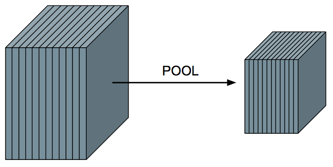
This layer is primarily used to help reduce the computational complexity and extract prominent features. The pooling layer, symbolized as POOL, has no weights/parameters, unlike the CONV layers. The result is a smaller activation volume along the the width and height. The depth of the input is still maintained, e.g., if there are 12 activation maps that go into a POOL layer, the output will also have 12 activation maps.

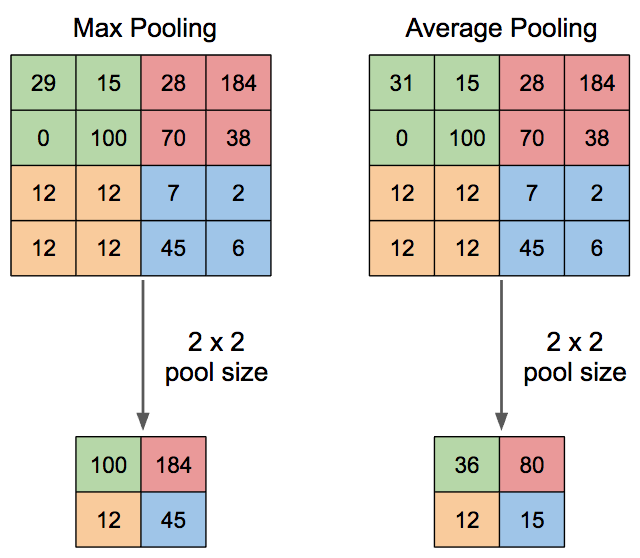
For POOL layers, we have to define a pool size, which tells us by how much we should reduce the width and height of the activation volume. For example, if we wanted to halve the input activation volume along both width and height, we would choose a pool size of 2×2. If we wanted to reduce it by more, we choose a larger pool size. The most common pooling size is 2×2. The below figure shows how the pools are arranged. We take a little window the size of the pool, perform some computation, and then slide it over so it doesn’t overlap and repeat.

The computation we do depends on the type of pooling: average or max.

For max pooling, inside of the window, we just choose the maximum value in that window. This intuitively corresponds to choosing the most prominent features. For average pooling, we take the average of the values in the window. This produces smoother results than max pooling.

In practice, max pooling is used more frequently than average pooling, and the most common pooling size is 2×2.

Fully-Connected Layer

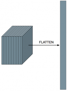
This layer is just a plain-old artificial neural network! The catch is that the input must be a vector. So if we have an activation volume, we must flatten it into a vector first!

After flattening the volume, we can treat this layer just like a neural network! It is okay to flatten here since we’ve already passed through all of the CONV layers and applied the filters.

Putting it all Together: The LeNet-5 Architecture

Now that we’ve discussed each of the layers independently, let’s revisit the LeNet-5 architecture.

(Gradient-Based Learning Applied to Document Recognition by LeCun et al.)

The above figure isn’t directly applicable to our case. The inputs we’ll be dealing with are actually 28x28x1. But we can still perform a convolution so that the resulting volume is 28x28x6 by using some zero padding. We perform a convolution with 6 feature maps to get a resulting activation volume of 28x28x6. These filters will be 5×5. Then we subsample/pool to get 14x14x6 activation volume: we’ve halved the width and height so we use a pooling size of 2×2. Then we convolve again with 16 feature maps to get the activation volume of 10x10x16, meaning we must have used filters of size 5×5 (as an exercise, double-check this in the convolution equation). We pool again with a pooling size of 2×2. The last convolutional layer is 120 filters of size 5×5, which also flattens our activation volume into a vector. If it wasn’t, then we would have to flatten it, which usually is the case. Finally, we add a hidden layer with 84 neurons and the output layer with 10 neurons.

The output layer neurons produce 10 numbers, but they don’t really mean anything, so it would be better for our understanding to convert them into something interpretable like probabilities. We can use the softmax function to do this. Essentially, it takes the exponential of each of the 10 numbers and scales them by the sum of the exponentials of all of the numbers to make a valid probability distribution. Now we can interpret the output as a probability distribution! When we backprop, this softmax distribution is more useful than just a plain max function.

Now that we understand each of the pieces, let’s start coding!

Coding LeNet-5 for Handwritten Digits Recognition

Since these layers are a bit more complicated than the a fully-connected layer, we won’t be coding them from scratch. In real applications, we rarely do this for fundamental layers. We use a library to do this. Keras is a very simple, modular library that uses Tensorflow in the background and will help us build and train our network in clean and simple way.

First, we need to load the MNIST dataset. Keras can actually help us do this by calling a single function. If the dataset hasn’t been downloaded yet, Keras will download it for us; if it has, Keras will load it and split it into a training and testing set.

import numpy as np
import keras
from keras.datasets import mnist
from keras.models import Sequential
from keras.layers import Dense, Dropout, Flatten
from keras.layers import Conv2D, MaxPooling2D

BATCH_SIZE = 128
NUM_CLASSES = 10
NUM_EPOCHS = 20

(X_train, y_train), (X_test, y_test) = mnist.load_data()

However, the data isn’t the right shape for our CNN. If we look at the shape of the training inputs, we see that they have the shape $60,000\times 28\times 28$ . The first dimension is the size of the training set, and the second and third are the image size. But we need to add another dimension to represent the number of channels. Numpy has a quick way we can do this.

X_train = X_train[..., np.newaxis]
X_test = X_test[..., np.newaxis]

Now our shape will be $60,000\times 28\times 28\times 1$ for the training input and $10,000\times 28\times 28\times 1$ for the testing input. This conforms with our CNN architecture! In general, the input shape usually has the batch size/number of examples, the image dimensions (width and height), and the number of channels. Be careful though, since sometimes the number of channels occurs before the image size (Theano does this) and sometimes it occurs after (Tensorflow does this).

There’s some additional image processing cleanup we can do by rescaling so that each pixel value is $[0, 1]$ .

X_train = X_train.astype('float32') / 255
X_test = X_test.astype('float32') / 255

As for the ground-truth labels, they’re numbers, but we need them to be one-hot vectors since we’re doing classification. Luckily, Keras has a function to automatically convert a list of numbers into a matrix of one-hot vectors.

y_train = keras.utils.to_categorical(y_train, NUM_CLASSES)
y_test = keras.utils.to_categorical(y_test, NUM_CLASSES)

Now its time to build our model! We’ll be following as close to LeNet-5 as possible, but making a few alterations to improve learning. To build a model in Keras, we have to create a Sequential class and add layers to it.

model = Sequential()
model.add(Conv2D(6, (5, 5), activation='relu', padding='same', input_shape=(28, 28, 1)))
model.add(MaxPooling2D((2, 2)))
model.add(Conv2D(16, (5, 5), activation='relu'))
model.add(MaxPooling2D((2, 2)))
model.add(Conv2D(120, (5, 5), activation='relu'))
model.add(Flatten())
model.add(Dense(84, activation='relu'))
model.add(Dense(NUM_CLASSES, activation='softmax'))

For the first layer, we have 6 filters of size 5×5 (with some zero padding) and a ReLU activation. (Keras also forces us to specify the dimensions of the input excluding the batch size). Then we perform max pooling using 2×2 regions. Then we repeat that combination except using 16 filters for the next block. Finally, we use 120 filters. In almost all cases, we would have to flatten our activation maps into a single vector. However, LeNet does not need to do this since at the last CONV layer, the size of the input activation map is already 5×5 so we would get a vector out anyways. Then we add an FC (or hidden) layer on top of that and finally the output layer.

We’re finished! Now all that’s left to do is “compile” our model and start training!

model.compile(loss='categorical_crossentropy',
              optimizer='adam',
              metrics=['accuracy'])

model.fit(X_train, y_train,
          batch_size=BATCH_SIZE,
          epochs=NUM_EPOCHS,
          validation_split=0.10)

The categorical cross-entropy is a different loss function that works well for categorical data; we won’t get to the exact formulation this time. As for the optimizer, we’re using Adam (by Kingma and Ba) since it tends to converge better and quicker than gradient descent. Finally, we tell Keras to compute the accuracy. There are other metrics we could compute, but accuracy will suffice for our simple case (Keras will always compute the loss).

After our model has trained, we can evaluate it by running it on the testing data.

score = model.evaluate(X_test, y_test)
print('Test accuracy: {0:.4f}'.format(score[1]))

Expect to see a score in the high 90%’s! That’s why CNNs are so awesome at vision tasks!

During training Keras will helpfully display the progress like this.

Using TensorFlow backend.
Train on 54000 samples, validate on 6000 samples
Epoch 1/20
54000/54000 [==============================] - 9s - loss: 0.3757 - acc: 0.8864 - val_loss: 0.1183 - val_acc: 0.9662
Epoch 2/20
54000/54000 [==============================] - 9s - loss: 0.1049 - acc: 0.9676 - val_loss: 0.0779 - val_acc: 0.9770
Epoch 3/20
54000/54000 [==============================] - 9s - loss: 0.0709 - acc: 0.9782 - val_loss: 0.0675 - val_acc: 0.9807
Epoch 4/20
54000/54000 [==============================] - 9s - loss: 0.0554 - acc: 0.9824 - val_loss: 0.0597 - val_acc: 0.9830
Epoch 5/20
54000/54000 [==============================] - 9s - loss: 0.0437 - acc: 0.9863 - val_loss: 0.0429 - val_acc: 0.9877
Epoch 6/20
54000/54000 [==============================] - 9s - loss: 0.0364 - acc: 0.9889 - val_loss: 0.0407 - val_acc: 0.9877
Epoch 7/20
54000/54000 [==============================] - 9s - loss: 0.0302 - acc: 0.9904 - val_loss: 0.0481 - val_acc: 0.9868
Epoch 8/20
54000/54000 [==============================] - 9s - loss: 0.0276 - acc: 0.9911 - val_loss: 0.0399 - val_acc: 0.9885
Epoch 9/20
54000/54000 [==============================] - 9s - loss: 0.0236 - acc: 0.9919 - val_loss: 0.0406 - val_acc: 0.9880
Epoch 10/20
54000/54000 [==============================] - 9s - loss: 0.0197 - acc: 0.9938 - val_loss: 0.0419 - val_acc: 0.9872
Epoch 11/20
54000/54000 [==============================] - 9s - loss: 0.0189 - acc: 0.9936 - val_loss: 0.0368 - val_acc: 0.9895
Epoch 12/20
54000/54000 [==============================] - 9s - loss: 0.0151 - acc: 0.9948 - val_loss: 0.0438 - val_acc: 0.9873
Epoch 13/20
54000/54000 [==============================] - 9s - loss: 0.0154 - acc: 0.9949 - val_loss: 0.0468 - val_acc: 0.9870
Epoch 14/20
54000/54000 [==============================] - 9s - loss: 0.0121 - acc: 0.9960 - val_loss: 0.0411 - val_acc: 0.9892
Epoch 15/20
54000/54000 [==============================] - 9s - loss: 0.0123 - acc: 0.9955 - val_loss: 0.0447 - val_acc: 0.9877
Epoch 16/20
54000/54000 [==============================] - 9s - loss: 0.0097 - acc: 0.9968 - val_loss: 0.0538 - val_acc: 0.9867
Epoch 17/20
54000/54000 [==============================] - 9s - loss: 0.0101 - acc: 0.9965 - val_loss: 0.0457 - val_acc: 0.9887
Epoch 18/20
54000/54000 [==============================] - 9s - loss: 0.0080 - acc: 0.9974 - val_loss: 0.0473 - val_acc: 0.9893
Epoch 19/20
54000/54000 [==============================] - 9s - loss: 0.0105 - acc: 0.9964 - val_loss: 0.0540 - val_acc: 0.9858
Epoch 20/20
54000/54000 [==============================] - 9s - loss: 0.0087 - acc: 0.9972 - val_loss: 0.0482 - val_acc: 0.9890
 9760/10000 [============================>.] - ETA: 0s
Test accuracy: 0.9894

To recap, we discussed convolutional neural networks and their inner workings. First, we discussed why there was a need for a new type of neural network and why traditional artificial neural networks weren’t right for the job. Then we discussed the different fundamental layers and their inputs and outputs. Finally, we use the Keras library to code the LeNet-5 architecture for handwritten digits recognition from the MNIST dataset.

Convolutional Neural Networks are at the heart of all of the state-of-the-art vision challenges so having a good understand of CNNs goes a long way in the computer vision community. It also goes a long way in terms of developing your skills for professional Python development – so make sure you’re comfortable with using CNNs!