You can access the full course here: Bite-Sized Pandas
Part 1
In this lesson we’ll learn about DataFrames (the data structure pandas works with) and learning how to access data in the DataFrame using pandas.
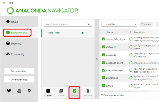
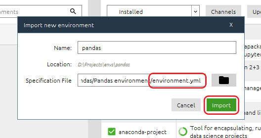
We’ll open Anaconda Navigator and load our environment file.
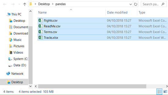
Now we need to copy the files we’ll be working with into your working directory – maybe create a folder specifically for this course. The files we’ll use are flights.csv, ReadMe.csv, Terms.csv and Tracks.xlsx.
Now we can get started with pandas!
In Anaconda Navigator make sure you have the pandas environment selected before launching Spyder.
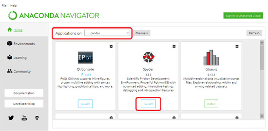
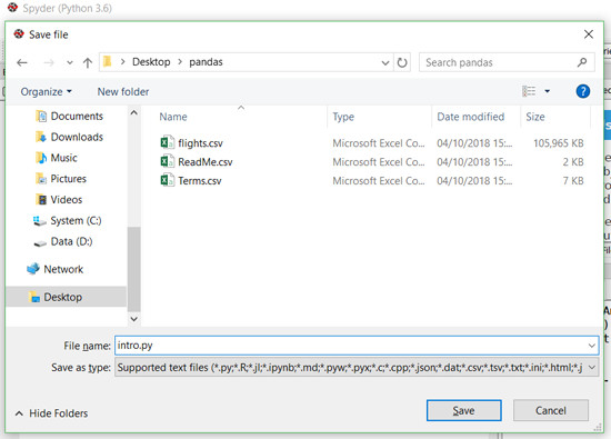
Save your new file in the same directory as the spreadsheets so they’ll be easy to access.
Now we’ll start by importing pandas, and then numpy, which we’ll use to populate data.
import pandas as pd
import numpy as np
Creating a DataFrame:
A DataFrame is a like a spreadsheet – a 2D table with rows and columns, very similar to a spreadsheet you’d open in Excel. Using pandas gives us a lot more power behind how we can work with them.
Let’s start by creating a DataFrame from data we have.
Remembering it’s a 2D table, a way we can define a DataFrame is to make a dictionary first, then give that to pandas to convert into a DataFrame. So let’s make a python dictionary. Usually we use df to mean DataFrame:
df_data = {

}
Within this dictionary, each key will be a column, with their values being the row data in that column.
To see how this looks, let’s populate a column with some random values using numpy.
df_data = {
'col1': np.random.rand(5)
}
This will generate a single column with 5 rows. Let’s convert it to a DataFrame to see what it looks like before we add more columns.
df = pd.DataFrame(df_data)
print(df)
If you run this, you’ll see our DataFrame printed to the console populated with 5 random values thanks to numpy.
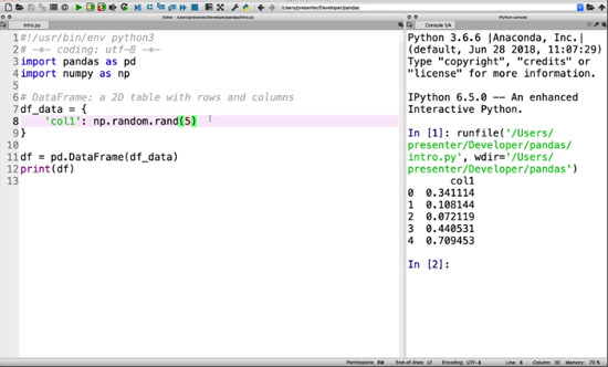
Let’s go ahead and make another couple of columns and run it again:
df_data = {
'col1': np.random.rand(5),
'col2': np.random.rand(5),
'col3': np.random.rand(5)
}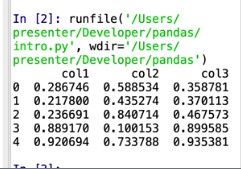
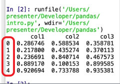
Now you can see how we can give data to pandas in the form of dictionaries and how they’ll look when converted into DataFrames, including how pandas automatically indexes our rows for us.
Fetching Rows:
We can deal with it much like you would a list, using indices to return the values we want. Try printing only the contents of the first 2 rows.
print(df[:2])
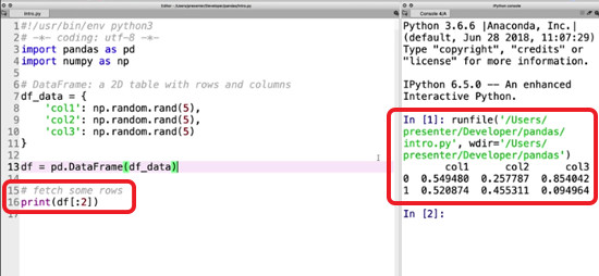
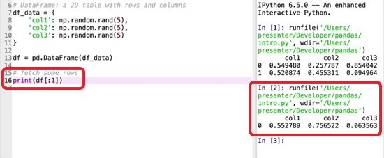
Remember: indices start at 0 and go up to but don’t include the final stated index. So if we only wanted the first row, we would use [:1].
Fetching Columns:
This is only slightly different – instead of numbered indices, we refer to the column’s name. Change your print command to fetch all the data from the first column only.
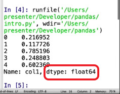
print(df['col1'])

You’ll see it also helpfully returns the type of data contained in that column’s rows.
Documentation:
Go to https://pandas.pydata.org/ and click on the documentation link.
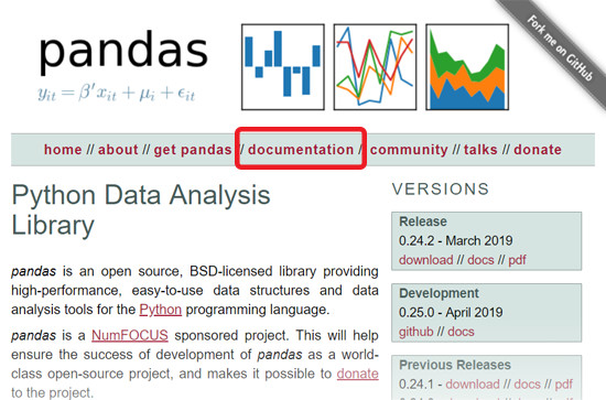
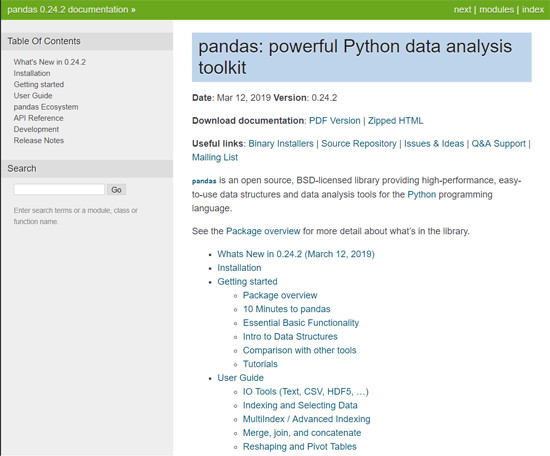
Here we have all the documentation we need to understand and use pandas. If you’re ever stuck, try here!
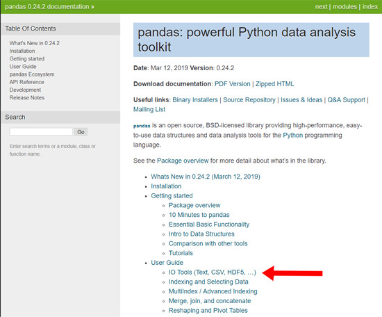
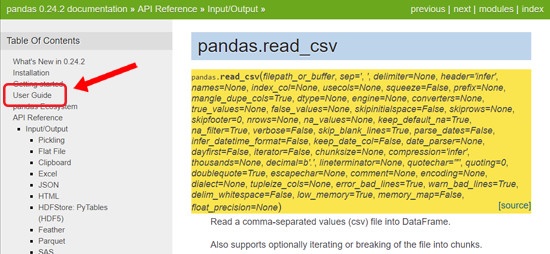
Under User Guide, click on IO Tools (Text, CSV, HDF5, …), and you’ll find all the functions that we can use to read CSV files.
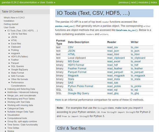
Now if you click on any function, say, pandas.read_csv()…
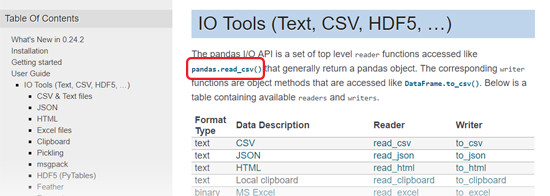
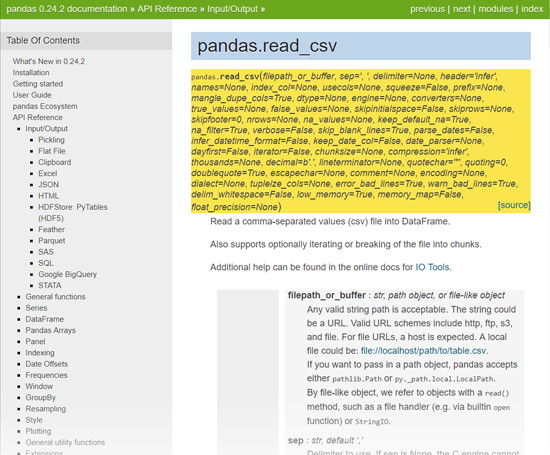
You can see all of its specific documentation, explaining what you can do and how. In this case, pandas.read.csv() starts with a filepath_or_buffer, and then has all kinds of other information you could use to customize that function.
Elsewhere in the User Guide there are sections that can also help you with using pandas to read from JSOM, Excel or HDF5, and more! There’s also a search bar under the Table of Contents so you can search for specific function names, so if you ever get stuck or want to improve your pandas skills, this is a great place to start!
Challenge:
This challenge will help you get used to using the pandas documentation to solve problems.
Your aim is to select multiple columns from the DataFrame we made – columns 1 and 2.
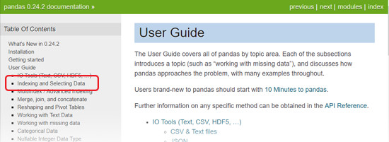
Clue: When looking in the documentation, the answer will be somewhere near the top of the page called Indexing and Selecting Data. Try to figure out how to do this on your own before reading on.
Solution:
In case you didn’t find it, the part of the documentation you need is under the subtitle Basics and begins “You can pass a list of columns to [] to select columns in that order.”
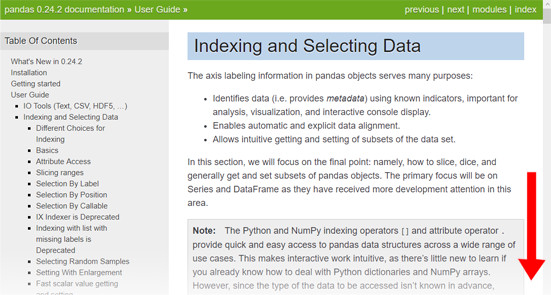
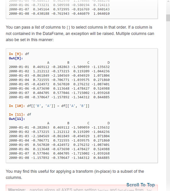
In the above example, columns B and A and selected and the data in their rows are swapped.
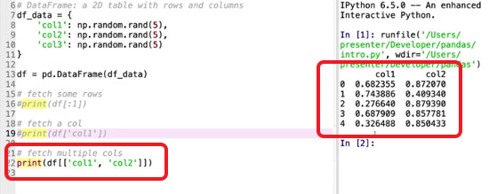
So, to get the data from multiple columns, instead of a string, we can use a list:
print(df[['col1', 'col2']])
Part 2
In this lesson we’ll learn how to read data from CSV and Excel into Pandas and save as a Pandas data file.
There’s a function in Pandas that we can use for this that’s easy to use and handles all of the formatting needed – all we have to do is give it a file name!
Make a new file in Spyder in the same directory as the project files.
Start by loading Pandas:
import pandas as pd
Next we’ll have Pandas read an Excel spreadsheet. Open Tracks.xlsx in Excel and let’s have a look at what we’ll be working with first.
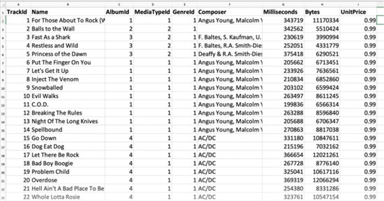
We can see that it’s a list of songs with various related data, such as album ID, Artist and price.
The Pandas function we’re using is read_excel, and we want it to load the file Tracks.xlsx.
tracks = pd.read_excel('Tracks.xlsx')We may also need to choose which sheet within the Excel Workbook we want to load, as we can only load one sheet per DataFrame. If you have multiple sheets, you’ll need to create multiple DataFrames, each utilizing this function. If we don’t specify which we want, it’ll select the first sheet by default.
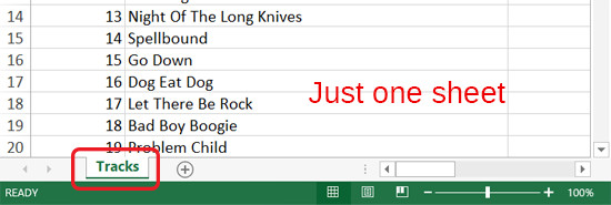
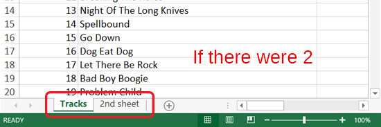
We can specify which sheet either by using the actual name of the sheet or using a zero-indexed integer. In this case there is only one sheet in the workbook so it’s not necessary, but it’s worth practicing!
tracks = pd.read_excel('Tracks.xlsx', sheet_name=0)
print(tracks)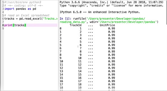
There’s a lot of data here! In addition to printing our sheet, this tells us how many rows and columns the sheet has.
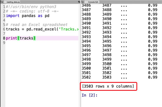
Pandas seems to have removed the middle columns and rows, but it hasn’t actually. This is purely for display purposes to make it easier for us given the quantity of data we’re working with – the data is still there, don’t worry! This is obviously very convenient given that our sheet has over 3,500 rows!
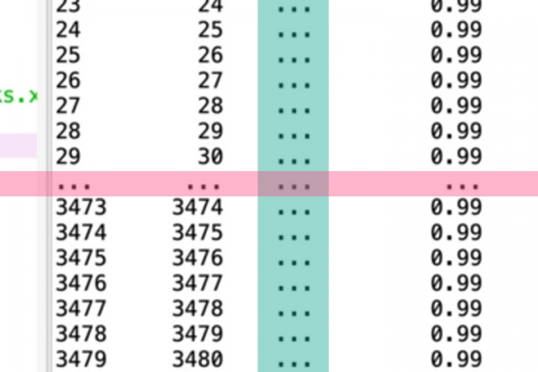
If you’re ever concerned, you can ask for those missing columns and rows. Let’s do that now by printing the columns.
print(tracks.columns)
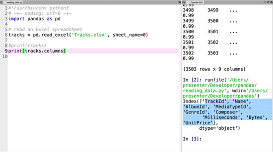
We can now see that it has all the columns we wanted. We can make extra sure by asking for the contents of an individual column. Let’s print out the milliseconds column:
print(tracks['Milliseconds'])
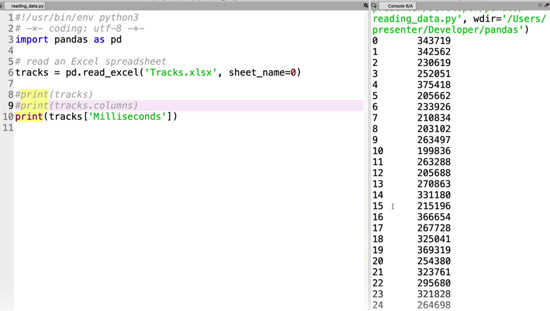
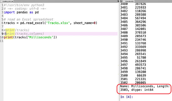
And there it is, abbreviated as before with dots in the middle, and with some helpful information at the bottom: the name of the column, the number of rows, and the data type.
Now let’s do the same with a CSV spreadsheet – flights.csv. Have a look at it before if you like. It contains lots of information about flights during 2017. Instead of read_excel, we’re using read_csv – other than that it’s exactly the same:
flights = pd.read_csv('flights.csv')
print(flights)
Run this. You may have to wait a little – it’s a big file!
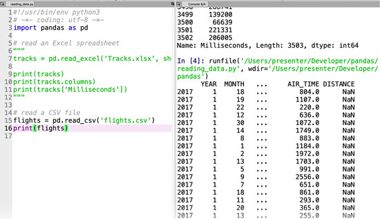
You’ll notice that we have a similar issue. With 600,000 rows and 25 columns, the data we actually have printed out is reduced nicely. That’s good, but there seems to be a problem – the data isn’t matching up with the column names.
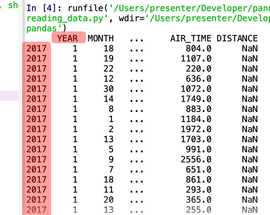
This is because when we load a CSV like this in Pandas, unlike with Excel files, it will try to use the first column as the index, which is why everything’s been offset by one. To resolve this, we need to add a parameter:
flights = pd.read_csv('flights.csv', index_col=False)
print(flights)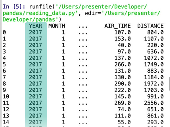
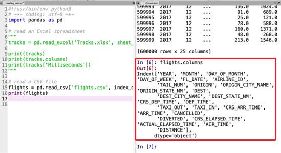
Fixed! Once again, if we want to check on those apparently missing rows and columns we can.
print(flights.columns)
Transcript 1
Hello world and thanks for joining me. My name is Mohit Deshpande and in this course, we’re going to be learning how to manage and analyze data using PANDAS, a library called PANDAS for data analysis.
So we’re gonna learn a lot about how we can read-in data from sources, and then manipulate it so we can use it for further data analysis. So some of the things that we’re going to be learning about in this course, is we’re gonna learn about DataFrames, which are how we can store data in PANDAS so we can later use them for any kind of analysis. We’ll learn how to read information from CSV files and Excel files. We’ll learn all about how to select, sort, filter our data and then we’re also gonna get into how we can do different kinds of grouping and data aggregation as well.
So we’re gonna be learning a lot of different things that center around this library data science, and data analysis library called PANDAS, and we’re gonna really learn how to use this, so that we can do further data analysis on the data that we have.
We’ve been making courses since 2012, and we’re super excited to have you on board. Online courses are a fantastic way to learn new skills, and I take a lot of courses myself. Zenva courses consist mainly of video lessons that you can watch and re-watch as many times as you want. We also have downloadable source code and project files and they contain everything that we build in the lessons. It’s highly, highly recommended that you code along with me. In my experience, it’s the best way to learn something is to kinda get your feet wet or get your hands dirty.
And lastly, we’ve seen that the students who get the most out of these online courses are those that make some kind of weekly plan, and stick with it, depending of course on your own availability and learning style. So Zenva over the past six years has taught all different kinds of topics on programming and game development. Over 300,000 students, over 100 courses. The skills that they learn in these courses are completely transferrable to other context and domain. In fact, some of the students have used the skills that they learned in these courses to advance their own careers, to make a startup, or to publish their own content from the skills that they’ve learned.
Thanks again for joining, and I look forward to seeing all the cool stuff you’ll be building. Now without further Ado, let’s get started.
Transcript 2
In this video we’re going to get started with Pandas, and so learn a little about what the fundamental data structure for Pandas is as well as learning how to access a data using a thing called data frame. But first of all what we’ll need to do is download the source code and we’ll need to copy them into whatever working directory on your computer. ‘Cause inside here we have these files that we’ll need. So you’ll have to copy these files over into your working directory. So I’ve already done this and created a folder called Pandas and I’ve copied over all of these things that we’ll need.
You’ll want to open up your Anaconda Navigator and make sure you have the right environment selected and then we’re going to launch Spyder. Okay, so lets get started. So we’ll need to import Pandas, import Pandas as pd. And I’m also going to import NumPy as np just so that we’re going to use it to populate data.
We’re gonna talk a little bit about Pandas, what the fundamentals data structure behind Pandas is. And the thing is called a DataFrame. And a DataFrame you can think of it as just being a single spreadsheet. A 2D table with rows and columns. So let’s just create a DataFrame from just some data that we have. So remember it’s a 2D table. So how I can define a dataframe is I can use a dictionary first, then give it to Pandas and say Hey, can you convert this dictionary into a dataframe. Each of the keys are going to be columns and the values are going to be rows. Column one, now I can just populate it with some random values, np.random.rand five.
Essentially what I have done is created a single column and it has five rows. So let’s just create this dataframe first so that we can see it. df equals, I can just create one by saying pd.DataFrame and I just pass it in this dictionary. Pass in now I’ve created a DataFrame. Let’s see what this looks like. I can run this guy and you’ll see I have column one and then just some random garbage values. So let’s go a head and create another column, create another one and you’ll see now we have three columns. And so this is just how we can give into or you can give data to Pandas into a dataframe just by using this dictionary where the keys are the columns and the values are going to be the actual values for that column.
We’ll see if we can fetch some rows and how we can fetch some columns. Index it like you would a list. So I’ll say, let’s get some, I’ll run this and you’ll see that we’ll get the first two rows because remember that this goes, we start at zero and we go up two but not including this index. So we get zero and one. Instead we need to see what the column name is. So let’s do col1 and what that will do is when I run it print out all of the rows the entire column, all the rows for this particular column and it even goes so far as to tell me the data type. In order to fetch multiple columns we actually use a list inside here.
Suppose I want to fetch the first two column I can say something like print df and then inside of here instead of doing just quotes here I can do a list, I’m indexing and I’m giving it a list to index on. So I can say col and col2. So now if you see we have extracted two columns.
Transcript 3
In this video we are going to learn how we can read data from CSV and excel into pandas, into a panda’s data frame. First thing only to do is import pandas. Alright so let’s load in, let’s read an Excel spreadsheet, and to give you an idea of the kind of the data that we’re going to be loading I have the spreadsheet opened up in excel so it’s just a list of different songs.
So I’ll say tracks equals and then I just call pd.read_excel and then I can just give it a file name, so I know this that the file is called Tracks.xlsx, so this will just load our data, so it’s really this simple to load data into Panda. So let’s print this guy out and see for ourselves, so you can see that I have some data here, and it’s actually already telling me how many rows and columns I have. So because we can’t see all of the columns here let’s print out the columns just so we can verify that they’re there, so I comment this out. I’m going to say tracks.columns and we can print out.
We can print out all of the columns, so I can run this and see that we can see all of the columns that are being printed out, and additionally what I can do, and now that I have this information you know I can do something like, let’s print out all of the entire column that’s milliseconds and just do something like this, and then it’ll print out all of the milliseconds and it’s giving me some useful information, like the name of the column is, how many rows we have and then what the data type.
What we can do is see how we can read a CSV, so I can load this guy up just by saying pd.read_csv and I have to give it the CSV file, so flights.csv and then we can do the same thing let’s just print this out just so that we can have some idea of what’s going on. But you can see that we have 600,000 rows and then 25 columns, so it’s a pretty big data set. If we can see if I can expand this out a little bit, alright so it’ll say year, month, but wait a minute this isn’t quite right, cause this should be the year, so it seems all the columns are offset by one. So this isn’t good, and this is because when we’re loading something like this in Panda is what it’s going to try to do is find, use this first column as the index, and we don’t want it to do that.
We want to just have natural, natural indexes, so just zero, one, two, three and so on, and so on. So what I can do is just use a parameter here and say index_col=False, and so now let me run this. Alright so now let’s see what we have. So okay, this seems to be, this seems to be promising alright, so this is the correct column for the year.
This is the correct column for the months, so month one being January, and now you got the indexes are correct so it’s zero up to 59,999 because remember it’s zero index. Flights.columns and we can see all of the columns, so that’s how we can read excel and CSV spreadsheets in Pandas.
Interested in continuing? Check out the full Bite-Sized Pandas course, which is part of our Bite-Sized Coding Academy.


