You can access the full course here: Probability Foundations for Data Science
Part 1
In this lesson, we’re going to see an introduction to the Probability Theory.
Probability definitions
We define probability as the likelihood of some event happening.
For coin flipping, there is an equal probability of having heads or tails (1/2 each), and we represent it by the following expression:

Probability is usually represented by “p” and the event is denoted with a capital letter between parentheses, but there’s not really a standard notation as seen above.
The event, in turn, is some sort of action that has a probabilistic outcome. In the case of a coin, we do not know what the outcome is until we’ve flipped it.
Dice toss is another classic example where, for a 6-sided dice, we have a 1/6 chance of the dice landing on any particular side.
Now, the probability of the dice landing on an even number, however, is equal to 3 (as there are 3 even numbers in the range 1-6) divided by the total number of sides (6):

In general, here’s how we compute the probability of an event E happening:

All probabilities go from a chance of zero to one, and a good way of understanding this is as shown below:
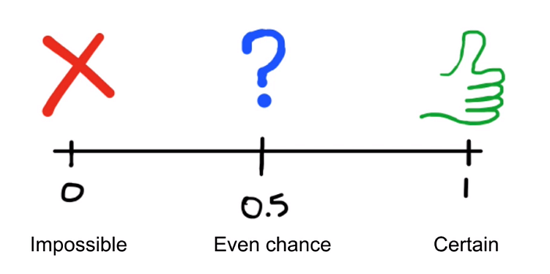
All probabilities will never be less than zero or greater than one.
There’s also the notion of the complement of an event, which basically consists of outcomes not in the event. It can be written in various different ways:

Let’s move to an example to better understand the concept of complement:
Suppose we want to compute the probability that a dice roll is not one. That is the same as the sum of the probabilities of it being numbers two, three, four, five and six (all other numbers but number one):

Another way to compute the complement is by doing 1 minus the probability of the actual event. So that, given any probability, we can immediately compute the probability of it not happening (that is, its complement) by computing its difference to 1.
Dice event probability and its complement
Let’s compute the probability of the outcome of a roll of a dice being strictly greater than 4. Well, in that case, we have two possibilities (sides 5 and 6 of the dice). It results in 2 outcomes out of the 6 total possible outcomes, which can be reduced to a chance of 1/3:

Computing the complement of this event we have 2/3, which is easily done by the definition of complement (namely 1 – 1/3):

It is important to notice that the probability of a given event added to the probability of the complement of this same event will always add up to 1.
Now that we’ve seen the basic definitions of probability, let’s move on to the next lesson.
Part 2
We are now going to use Pandas to do some probability computations.
Setup
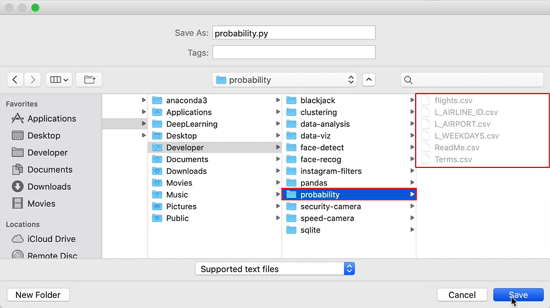
To get started we’ll be using the following files:

There are a bunch of CSV files here, where the one called “flights.csv” is the main dataset we are going to work with. It has a little over half a million U.S. domestic flights from the year 2017, containing all kinds of information about the flights, such as origin city, origin state, destination city, destination state, flight airline, distance of the flight, departure and arrival times, and so on.
File “ReadMe.csv” explains in more detail the different columns of “flight.csv”:
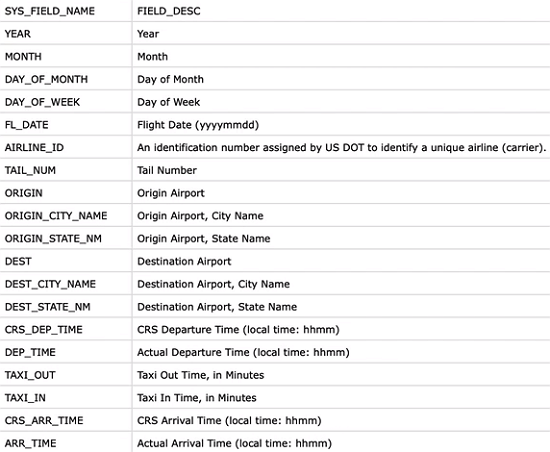
There are also additional files (“L_AIRLINE_ID.csv”, “L_AIRPORT.csv”, and “L_WEEKDAYS.csv”) containing airline, airports, and weekdays codes.
“Terms.csv” has flight-specific terminology, with several terms and their definitions for your aid. In case you are not familiar with any of the terms used in the other files, you can read this file. See part of its contents down below:
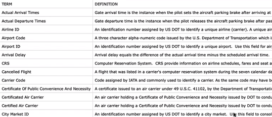
Now that we took a look at the files on our source code folder, we launch Spyder:

Save your Spyder running instance in the same folder you unzipped before, where the CSV files are:
Starting the code
We start our Python code by importing Pandas, and reading from our flights spreadsheet:
import pandas as pd

flights = pd.read_csv('flights.csv', index_col=False).dropna()
By calling the dropna function, Pandas reads our flights’ file and drops any line containing at least one missing value.
We first compute the probability of, given no other information, picking a random flight that started in California. To calculate it, if we go back to the definition of probability, we have to divide the total sum of flights starting in California by the total amount of flights in general.
For the first part of our equation, we need to find the total sum of flights originating in California:
num_flights_in_CA = (flights['ORIGIN_STATE_NM'] == 'California').sum()
To get the total amount of flights is pretty straightforward. We just need the length of our variable “flights”. It gives us the number of rows in “flights”:
total_flights = len(flights)
And then we print the result, which is the number of flights from California divided by the total amount of flights:
print('p(flight started in California) = {}'.format(num_flights_in_CA/total_flights))We see that the probability for a flight to start in California is about 13%:
p(flight started in California) = 0.13300369068719986
California was just an example, though. Let’s get a full probability distribution for all states in our flights’ file.
Full probability distribution
For every state, we want to compute the probability of a flight starting in that particular state. For that, we need to group the states by name:
flight_states = flights.groupby('ORIGIN_STATE_NM')We use Pandas function “size” to get a sum of the total number of flights for each individual state:
num_flights_per_state = flight_states.size()
We are just lacking the division for the number of all flights from the year 2017, done by an apply call, as follows:
flight_state_prob = num_flights_per_state.apply (lambda num_flights: num_flights/total_flights)
The lambda function applies the code to each state group.
Printing “flight_state_prob”, we have a list with all states and their calculated probabilities. See some of the probabilities:
Nebraska
0.004045
Nevada
0.029836
New Hampshire
0.001100
New Jersey
0.021017
New Mexico
0.003916
New York
0.042568
Finally, to find out what the maximum probability is and its corresponding state, we run:
print(flight_state_prob.max())
print(flight_state_prob.idxmax())
It turns out that the state with maximum probability as origin state of a randomly picked flight of all 2017 domestic U.S. flights is, in fact, California (with its 13% probability).
So this introduced us to how to perform some basic probability operations using Pandas.
You can find Pandas documentation here: http://pandas.pydata.org/
Transcript 1
Hello world and thanks for joining me. My name is Mohit Deshpande. In this course, we’ll be learning all about probability theory and building a naive Bayes classifier that will be able to predict if our flight will land late or not. We’re gonna be learning all about probability in this course.
The first thing that I wanna do is introduce you to the concept of probability, if you’re not already familiar with it and just to get all of the rotation out of the way. Then we’re gonna move on to conditional probability and that’s kinda the backbone of a lot of machine learning and data science algorithms that’s working. Having a good idea of conditional probability will also help you out in a ton of other fields as well.
Next we’re gonna move on to Bayes’ theorem which is gonna follow from a conditional probability. And Bayes’ theorem, again, is a very fundamental statistical theorem that’s used in all kinds of different applications. One application in particular is using it in a naive Bayes classifier. We’re gonna build a naive Bayes classifier that we’re gonna train it on a data set of flights and see if we can predict whether a flight will land late or not, given some set of features, such as how long the flight is in the air, the distance between the two airports, their departure time, the airline, and so on and so on.
We can experiment with the groupings of features to see if we can get a really accurate classifier. We’ve been making courses since 2012 and we’re super excited to have you onboard. Online courses are a great way to learn new skills and I take a lot of online courses myself.
Zenva courses consist mainly of video lessons that we can watch and rewatch at your own pace as many tines as you want. We also have downloadable source code and project files and they contain everything that we build in the lessons. It’s highly recommended that you code along with me. In my experience, that is the best way to learn something new, is to get your hands dirty.
Lastly we’ve seen that students who get the most out of online courses are those that make a weekly plan and stick with it, depending, of course, on your own availability and learning style. Zenva, over the past six years, has taught all kinds of different topics on programming and game development to over 300,000 students across over a hundred courses. The skills that they learn in these courses are completely transferrable to other domains.
In fact, some of the students that have used, have taken these courses, have used the skills to advance their own careers, to start a company or to publish their own content from the skills that they’ve learned. Thanks again for joining. I look forward to seeing all the cool stuff you’ll be building. Now without further ado, let’s get started.
Transcript 2
In this video, I want to introduce you guys to a little bit about probability theory and how to compute it and so that we can get sort of using it in many of our applications that we’re gonna be working on, so what we’re gonna talk about, let’s go through, gonna introduce probability just to make sure that everyone’s on the same page regarding things like notation and how to actually compute it, and then we’re gonna quickly move on to conditional probability, and thus on to Bayes theorem.
So Bayes theorem depends on having a knowledge of conditional probability and we’re gonna have lots of examples with all of this information as well, and then finally, we’re gonna culminate in knowing, we’re gonna be learning about the naive Bayes classifier and we’re gonna use it, apply it to a set of flights to see if we can predict if our flight is going to arrive late based on any number of given factors, so things like the distance between the two airports, what our departure time is, maybe the airline that we are flying, given all this information.
We’re gonna try to see if we can build a naive Bayes classifier that can predict if our flight is going to arrive late so it’s a really cool application of all the probability that we’re gonna be learning but we have to actually get started learning some of this probability, so I just wanna start off just introducing some concepts in probability and some notation, just so that everyone is on the same page. So probability is a likelihood of some event happening.
So I have two examples here, I have one involving a fair coin, one involving a six-sided dice. So if you think about a fair coin, a fair coin has two sides, and so there’s an equal chance or equal probability of the coin landing on heads or landing on tails if you flip it, and so here’s just some examples, some notation that we might use, so we have the probability that the coin lands on heads is gonna be equal to 0.5 or 1/2, and here’s some notation that you might encounter in other places if you see it, so sometimes probability is denoted as lowercase p and the event is gonna be in parentheses, sometimes, it’ll, especially with coins, sometimes just shortened to h or t.
Sometimes we capital p, sometimes we’ll write the full word Prob for probability but this is just some notation. We might see in many place, there is no standardized way of this notation. And speaking of events, so an event to just some kind of action that has a probabilistic outcome, so flipping a coin is an event, because we don’t know what the outcome is yet until we flip the coin. And the chance of the coin is 1/2 on each.
Again, a dice toss is another example of an event. There is a one in six chance of it landing on any one particular number, so if you roll a fair dice and it lands on three, the probability that it landed on that three is one out of six. We can do some more advanced, we can do a bit of more advanced problems, so we can just ask, what’s the likelihood that this dice lands on an even number? Well, how many even numbers are there on a six-sided dice, right, there’s two, four, and six, and how many different sides are there?
There are six. So three divided by six, 1/2 is equal to 0.5, so in general here’s how we compute probability of some event, e is quite simply just a number of ways that e can happen divided by the number of total possible outcomes of our event, so in the case of a coin toss, the probability of heads, there’s only one way that it can happen, lands on heads, the number of possible outcomes is two, because there is a heads and a tails, it could have landed on heads or tails, so just some precursor, this is just some information to just get everyone on the same page.
Speaking of probability values, all probabilities go from zero to one, including zero and one, so if you have something with a probability of zero, then we are saying that this event is impossible. If you have something with a probability of one, we are saying that this event is certain, and then somewhere in the middle, even chance is 50%. So it’s important to know that probabilities only range from zero to one, it doesn’t make sense for anything to have a probability greater than one or less than zero.
Okay, so one other concept that I want to just discuss is this notion of a complement of an event. So the complement of an event, and here are all the different ways that you can write it. Again, there’s no standard notation for this. You might see, you might as end up seeing all of these. The complement event, the complement of an event is all of the outcomes that are not in that particular event, so let’s do an example to get a better picture of what’s going on.
So suppose I wanna compute the probability that a roll of the dice is not one. So I want, so what are the different outcomes where the dice would not be one? Well, it turns out there are five, right? The dice can be two, three, four, five, or six. So there are five out of six and so I get end up with five six so that’s just kind of the complement of this, what it means for an event to have a complement. And we can compute it in another way. We just take the complement is equal to one minus the actual event, so here’s an alternate way of computing this. I can say, what is the probability that the dice is not equal to one is equivalent to saying what’s the probability of one minus the dice actually being one?
You can see that mathematically they equate to the same thing, but this is just an alternate way to compute a complement, so really given any probable, any kind of probability, we can immediately compute what’s the probability of this not happening just by taking one minus that one minus that number. All right, so let’s do just one more example to get this in your head.
So suppose I want to compute the probability that a roll of a dice is strictly greater than four. Well, outcome is that strictly greater four, it doesn’t include four, so the only two possible outcomes are five and six, so that’s two, two divided by how many outcomes, there are six, two divided by six and I should just reduce that to 1/3. Now I can say, I can take the complement of that event and if you use the formula, you can actually immediately compute it as being 2/3, because one minus 1/3 is 2/3.
So here’s just some notation of the probability that a dice is strictly greater than four, is equal to if I say what are the different outcomes of the dice not being strictly greater than four, well that means that the dice roll will have to be less than four, including four, and turns out, again, these are equivalent things here, so what is the likelihood that the dice lands on a number that’s less than four inclusive?
Well that’s gonna be one, two, three, four, four out of six possible outcomes, so that’s gonna be 2/3, so I can, there’s another way to compute this, if you have something like a dice or if you have a coin or some other kind of classic probability thing, classic probability object, classic probabilistic object if you wanna think of it that way, you can try to take the complement of an event and tie that into the actual geometry of the object itself, like what I’ve done here.
Alternatively, if I had something else, I would have to do the trick, the one minus trick to compute this output. Notice that all the numbers add up, all of them adds up, right, so the probability that a dice is strictly greater than four is gonna be one minus the probability that the dice is not strictly greater than four so it’s just gonna be one minus 1/3, and so that would be 2/3 and again, this is all this, all of this adds up.
So this hopefully is just a, this is really just to keep everyone on the same page when it comes to probability in terms of notation and how we actually compute probability, so hopefully this is just kinda giving you, it’s kinda quickly just giving you an idea of what probability is and how we’re gonna be using it in the future.
Transcript 3
So, what we’re gonna get started doing some probably computations on our dataset. So, the first thing you’ll need to do is go download the source code and then you’ll want to unzip it.
Make sure that you unzip it, and then put it somewhere. And if you go inside, I have a ton of CSV files and the main dataset that we’re gonna be working with, this is flights.csv, and it has a little over half a million US domestic flights from the year 2017. And that’s a kind of, that’s what we’re gonna be working with. It has all kinds of information about the flights, the origin, city origin, state, destination city, destination state, the flight id, the airline, the distance of the flight, the arrival/departure, the expected arrival/departure, and the actual arrival/departure time, and the time in the air, and all other kinds of information.
In fact, you can read all about the information in this ReadMe.csv. It shows you all of the different columns are as well as what they actually mean, and just for your curiosity, I have all of the information like airport codes, the airline codes, codes about week days, and as well as there’s some terminology, there’s a CSV sheet of terminology as well in case you’re unfamiliar with flight terminology. I certainly am not too familiar with it so I like to read through this as well.
So, please use all of these CSV files I have to your advantage so you get a better understanding of the dataset, so let’s get started. And so we’re gonna need to make sure we have the right environment and then launch an instance of Spider. And we actually have one running. And I’m just gonna save this as probability.pi inside of the same folder that houses the CSV files as well.
All right, so now we can get started and we’re gonna do some basic, we’re gonna do some basic probability computations. So, I’m gonna import pandas first. We’re gonna be needing that. Now I’ll just load in the data using pandas. Flight equals pd.read_csv flights.csv, index_col equals False, and then immediately we’re just gonna drop values that we’re not going to need. We’re gonna drop any no values or not a number. There are some but we just don’t wanna deal with them in our probability computation.
All right, I’m gonna write in comments the probabilities that we’re gonna be computing so that we get a better idea of how we can actually compute them. All right, so let’s start by computing the probability that with no other information, you just pick a random flight from the Air 2017, what is the probability that the flight started in California? I’ll just use the full code. What is the probability that the flight started in California?
Well if you go back to our definition of probability, we’re gonna have to compute the number of flights who’s origin state is California. Take the sum of all that and then divide by the number of total flights overall. So we can do that. So, num flights in CA equals, we can do flights, the column we’re looking for is Origin State Name. So I can get all the flights who’s origin state name is California. Then I’m gonna take the sum of all those. So this will give me all the flights that started in California.
Now I need to get the total flights and that’s also pretty easy to do really. We can just do something like lengths of flights. So let’s do len flights. And this just counts up the number of rows, and that’s total number of flights. And that’s all that there is. So, this is the probability so we can just print out this probability. We’re gonna say print. This is equal to dot format. You just divide these two numbers. So I’m gonna say this divided by total flights here.
All right, so this tells me, so let’s actually run this and see the results here. So after we run this, we see that the probability that any given flight started in the state of California is about 13 percent. Now, I just happened to pick California off the top of my head, but let’s get a full probability distribution for every state. So in other words, for every state I wanna compute the probability that the flight started in that particular state.
So I want to know the probability that a flight started in in New York, in California, in Wyoming, and Texas, and so on and so on. So I wanna compute the probability that a flight started in X for all states X. And then we can maybe do something like take a max operation and then figure out just looking at all the flights that happened in the past year, which was most probable in terms of which state you were leaving. So we can do that but what we’re gonna have to do is run an aggregate operation. I need to do a group by operation and then get the size of each group. So I can do that as well but what
I’m gonna leave as a bit of a challenge for you guys is to break down the line of code that would run a group by operation on this origin state name. So you’ll need to use the group by function in pandas to do that. Just go ahead and do that and we’ll be right back with the answer. Okay. So we’ll need to use what is called something like flight states equals flights dot group by then origin state name. So now we’ve grouped our flights by the state.
Now what we need to do is count up the number of flights in each state. So this is kind of like doing the sum operation here. So we can do that, we’ll say num flights per state. And there’s actually a convenient function for pandas that you might be aware of. This we just call dot size, will give us the number of flights in each group. ‘Cause since I’m grouping the flights by the state, I just need to basically run a count operation on each of those groups, and that’s what size does here, instead of having to use something like an apply function.
All right, so now I have the counts but I have the raw counts. Now what I need to do is actually divide by the total number of flights. And so I can do that just by running a simple apply operation. So, I can actually just print this. Or I should probably save it because we might want to do a max operation on it. So I’ll just say flight state probability is going to be the num flights per state, and what I’m gonna do is apply a function to this. So this is, again, a lambda function. In other words, the code that I’m gonna write here is gonna be applied to each group.
So, num flights. I just want to take each of the number of flights in a state num flights, I’m just gonna divide that by the total flights numbers. There’s just single number and I’m just taking each one of these groups and dividing it by total flights. That’s all that this is doing. And then we can print this out just to see. We’ll print this out to see the distribution of each. Of every state we’ll get a probability of what is the likelihood that if you pick any random flight from the year 2017, what is the likelihood that the origin was in this state? So let’s run this. Okay. So now we get this information right here.
So we can see that if you just pick any random state, Massachusetts, the probability of any one flight who’s origin was Massachusetts was about two percent. And again, we see a number here, about 13 percent in California, for example. But let’s get what the maxed is. So I can do that, I can just say print. We’re gonna say print the maximum, I’ll just say print max and that will give us a maximum value. But I want to– oops. I want to know which state that actually is. So I can print that out as well. I’m gonna comment this out. So then we run this. And we see that it turns out that California is actually the most likely state of your origin.
So if you pick a random flight in the past year, then odds are it’s most likely that the state was in California. Although that probability, again, it’s still quite small. It’s only about 14 percent. So this just kind of introduces us to performing some basic probability, computing some basic probability, using pandas and the different operations there. So just to recap where you can find the documentation for pandas. You go to pandas.pydata.org and click documentation.
There’s a ton of documentation if you need to refresh your memory on how to work with pandas here. So that’s all we’re gonna do in this video. So we just learned about how to perform basic probability operations using pandas.
Interested in continuing? Check out the full Probability Foundations for Data Science course, which is part of our Data Science Mini-Degree.


