An Overview of Reinforcement Learning: Teaching Machines to Play Games

Think back to the time you first learned a skill: driving a car, playing an instrument, cooking a recipe. Let’s consider the example of playing chess. Initially, it might have seemed difficult, but, as you played more and more, it became easier to understand the game. After playing many games of chess, you are much better than when you first started and “get” the game. You know which moves you should avoid and which moves you should play. In other words, you’ve developed experience by playing the game.

This is the same idea behind reinforcement learning. First, we’ll discuss what we need to define a game through a Markov Decision Process. Then we’ll discuss how we solve these using the Value Iteration Algorithm. We’ll discuss the Q-Learning algorithm for teaching a machine to play a game. Finally, we’ll implement Q-Learning in an OpenAI gym environment to teach a machine to play CartPole!

Download the full code here.

BUILD GAMES

FINAL DAYS: Unlock 250+ coding courses, guided learning paths, help from expert mentors, and more.

ACCESS NOW

Games

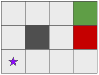
Before discussing reinforcement learning, we have to discuss the setup of a game. Before delving into the mathematics and definitions, let’s first try to use our reasoning. Suppose we have a robot (purple star) in an environment like the following picture.

The dark gray squares are walls. The green square yields the highest reward, e.g., the location of the buried treasure. The red square yields the lowest reward, e.g., a fire pit. We want to give commands to our robot to make it go to the green square and avoid the red square in the most efficient way possible. We have a finite number of actions: move left, up, right, and down. But, since we’re in the real world, the robot may not always go up. Robots don’t always act perfectly in the real world! Instead, our robot has a very high probability of doing the intended action, e.g., 90% chance of going up when we tell it go to up. However, there are non-zero probabilities that the robot will go in a different direction, e.g., 5% chance of going left or right when we tell it go to up. We have to keep these in mind when deciding which action to take.

These actions have to be taken within the confines of our environment, the most important characteristic of our game. Given our finite environment, there are only so many possibilities where our robot can be: the number of light gray squares. When we take an action, we go from one square to another, changing our board configuration. If we take the right actions, we can get to the green square and get a large reward!

Using the framework we described, we can define our game. Specifically, we use a Markov Decision Process (MDP) to define our game. An MDP is defined by the following.

1. Set of states
2. Set of actions that we can take at a state
3. Transition function where , , and that is nondeterministic because of real-world situations where we may not always follow the given action always.
4. Reward function that tells us what reward we get by taking action in state and ending up in state

Using these four things, we can define an MDP. The goal is to learn an optimal policy that tells us the optimal action to take at every state to maximize our reward.

We also introduce the concept of discounting: we prefer to have rewards sooner rather than later. We discount rewards at each time step so that we place an emphasis on having rewards sooner. This not only has a semantic meaning, but it is also mathematically useful: it helps our algorithms actually converge! Mathematically, we denote the discounting factor as . This will manifest itself in terms of exponential decay, but we’ll discuss that soon.

We can define these in terms of our robot in the environment. The set of states is all possible position of our robot. The set of actions is moving left, up, right, and down. We can model the transition function as being a probabilistic function that returns the probability of going into state after taking action in state . And the reward function can simply be a positive value if we go into the green square and a negative value for going into the red square.

Value Iteration

Knowing the transition function and reward function, the goal is to figure out the optimal policy . Value Iteration is technique we can use to solve for this. The idea is that we assign a value to each state that represents the expected reward of starting in and acting optimally. We have to compute an expected value because we’re not deterministic!

We can compute this using one of the Bellman Equations.

Let’s take a second to break this down. The sum is over all states and computes the expected reward of taking action in state . The in the front tells us to consider all actions and pick the expected reward that is the largest. Notice that we’re considering the discounting factor in the expectation. Also note that this definition is recursive: we have to know to compute .

Values near the high-reward states will have high values since there is a high expected reward because we’re close to a high-reward state and the discounting factor isn’t large. On the other hand, values far away from the high-reward state will have smaller expected reward because the discounting factor will be larger. Think of it this way: the farther you are, there are more chances for malfunctioning circuits in that distance as opposed to being right next to a high-reward state.

To compute these optimal expected rewards, we can use the Value Iteration algorithm. We initialize all for all states. And we compute the given all of the values of . Then, we compute  using  and so on using this equation.

We use this iterative Bellman equation to compute the next iteration of all of the values for all of the states given the previous values. Eventually, the values won’t change, and we say that the algorithm has converged.

Algorithmically, we can write the following.

1. Start with for all states
2. Compute
3. Go to Step 2 and repeat until convergence

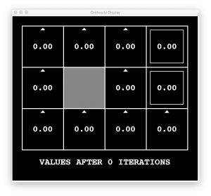
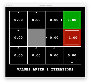
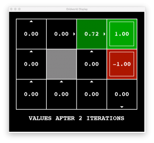
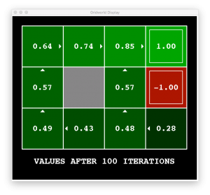
The amazing thing is that value iteration will certainly converge to the optimal values (I’ve omitted the exact proof). Here are some images that show value iteration for our robotic environment.

But remember our goal: find the optimal policy . How can we use these values to compute the optimal policy?

Suppose that we’ve run value iteration for a long enough amount of time, and our values have converged. In other words, we know for all states. To determine the policy, i.e., how to act at a state, we do a one-step lookahead to see which action will produce the maximum expected reward. This technique is called policy extraction.

Using value iteration and policy extraction, we can solve MDPs! However, we stated that we knew the transition and reward functions. In many real-world scenarios, we don’t know these explicitly! In other words, we don’t know which states are good/bad or what the actions actually do. Therefore, we can’t use value iteration and policy extraction anymore! We actually have to try to take actions in the environment and observe their results to learn. This is the heart of reinforcement learning: learn from experience!

Q-Learning

If we knew the transition and reward functions, we could easily use value iteration and policy extraction to solve our problem. However, in reinforcement learning we don’t know these!

Q-Learning is a simple modification of value iteration that allows us to train with the policy in mind. Instead of using and storing just expected reward, we consider actions as well in a pair called a q-value ! Then we can iterate over these q-values and computing the optimal policy is simply selecting the action with the largest q-value.

The q-value update looks very similar to value iteration.

We consider the expected reward, but we only look at the action that produces the largest q-value (). We can iterate over the q-values: the idea is to learn from each experience!

Here is the Q-Learning algorithm:

1. Perform an action in a state to end up in with reward , i.e., consider the tuple .
2. Compute the intermediate q-value
3. Incorporate that new evidence into the existing value using a running average (where is the learning rate). This can be re-written in an gradient-descent update rule fashion as 

Q-Learning, like value iteration, also converges to the optimal values, even if we don’t act optimally! The downsides of q-learning is that we have to make sure we explore enough and decay the learning rate.

Why do we want our agent to explore? If we find one sequence of actions that leads to a high reward, we want to repeat those actions. But there’s a chance that there exist another sequence of actions that could produce an even higher expected reward. In practice, we sometimes pick a random action instead of the optimal one a fraction of the time. This fraction is denoted by . The value of this encourages our agent to try doing some random values, i.e., to explore the state space more! This is called the -Greedy Approach.

Initially, our agent doesn’t know what to do or what actions lead to good rewards, so we start with a high value of (relatively) and decay it over time (because good actions become clearer as we play, and we should stop taking random actions). We may decay to zero, which means we should always take the optimal action after convergence. Or we can decay to a very small value, encouraging the agent to try random actions every once-in-a-while. The other parameter we decay is the learning rate, which will help our network converge to the optimal values.

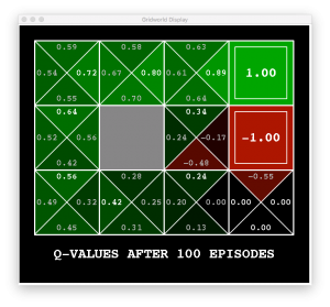
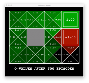
Here an example of running Q-Learning for our robotic environment.

Recall that the optimal policy is to take the action with the largest q-value at any state. If we did this for the above q-values, we would tend to go towards the higher reward and avoid the lower one.

Notice that there are some q-values that are still zero. In other words, we have arrived at a particular state where we haven’t taken a specific action. For example, consider the bottom-right square. We haven’t taken the down or right action in that state so we don’t know what value should be assigned to it.

Q-Learning Agent for CartPole

Now that we have an understanding of Q-Learning, let’s code!

Before starting, we’ll need to install OpenAI Gym (pip3 install gym ) and ffmpeg (brew install ffmpeg ). The OpenAI Gym provides us with at ton of different reinforcement learning scenarios with visuals, transition functions, and reward functions already programmed.

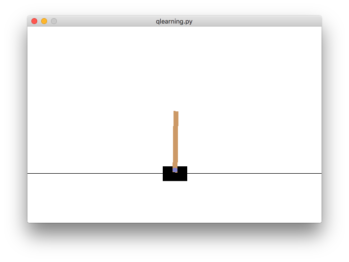
Now we’ll implement Q-Learning for the simplest game in the OpenAI Gym: CartPole! The objective of the game is simply to balance a stick on a cart.

This is a simple game that we can understand well. You can take the Q-Learning code we implement and generalize it to any of the games in the OpenAI Gym.

The state of this game is characterized by 4 quantities: position of the cart, velocity of the cart, angle of the pole, and angular velocity of the pole , respectively. But all of these quantities are continuous variables! We have to discretize the values by putting them into buckets, e.g., values between -0.5 and -0.4 will be in one bucket, etc. As for the actions, there are only two: move left or move right!

Let’s create a class for our Q-Learning agent.

import gym
import numpy as np
import math

class CartPoleQAgent():
    def __init__(self, buckets=(1, 1, 6, 12), num_episodes=1000, min_lr=0.1, min_explore=0.1, discount=1.0, decay=25):
        self.buckets = buckets
        self.num_episodes = num_episodes
        self.min_lr = min_lr
        self.min_explore = min_explore
        self.discount = discount
        self.decay = decay

        self.env = gym.make('CartPole-v0')

        self.upper_bounds = [self.env.observation_space.high[0], 0.5, self.env.observation_space.high[2], math.radians(50) / 1.]
        self.lower_bounds = [self.env.observation_space.low[0], -0.5, self.env.observation_space.low[2], -math.radians(50) / 1.]

        self.Q_table = np.zeros(self.buckets + (self.env.action_space.n,))

In the constructor, we use buckets to discretize our state space. In reinforcement learning, we train for a number of episodes, kind of like the number of epochs for supervised/unsupervised learning. We also have the minimum learning rate, exploration rate, and discount factor. Finally we have the decay factor that will be used for the learning and exploration rate decay.

We also bound the position and angle to be the same as the low and high of the environment. We manually bound velocity (0.5 m/s) and angular velocity (50 deg / s). Finally, we create the table of q-values.

In practice, we store all of the q-values in a giant lookup table. The rows are the state space and the columns are the actions. However, we characterized our state space as being a 4-tuple. So the resulting table will have 5 dimensions: the first four correspond to the state and the last one is the action index: . Given this tuple, we can access a scalar value in the table.

Speaking of the q-values, let’s write the code that will update a value in the table. Recall that the update formula is the following (substituting for .

We can translate this directly into Python code.

def update_q(self, state, action, reward, new_state):
    self.Q_table[state][action] += self.lr * (reward + self.discount * np.max(self.Q_table[new_state]) - self.Q_table[state][action])

Additionally, we’ll write update rules for the exploration and learning rates.

def get_explore_rate(self, t):
    return max(self.min_explore, min(1., 1. - math.log10((t + 1) / self.decay)))

def get_lr(self, t):
    return max(self.min_lr, min(1., 1. - math.log10((t + 1) / self.decay)))

This is just a form of decay. Essentially, we decay our exploration and learning rates until it is the minimum exploration and learning rate that we specified in the constructor.

We also need a function to choose an action using the -Greedy approach. percent of the time, we take a random action, but the rest of the time we take the optimal action. Recall that the optimal action is the following.

We can translate that into code.

def choose_action(self, state):
    if (np.random.random() < self.explore_rate):
        return self.env.action_space.sample() 
    else:
        return np.argmax(self.Q_table[state])

Now we can write some code to discretize our search space and train our agent! The first function simply does some math to figure out which buckets our observation should be in.

def discretize_state(self, obs):
    discretized = list()
    for i in range(len(obs)):
        scaling = (obs[i] + abs(self.lower_bounds[i])) / (self.upper_bounds[i] - self.lower_bounds[i])
        new_obs = int(round((self.buckets[i] - 1) * scaling))
        new_obs = min(self.buckets[i] - 1, max(0, new_obs))
        discretized.append(new_obs)
    return tuple(discretized)

def train(self):
    for e in range(self.num_episodes):
        current_state = self.discretize_state(self.env.reset())

        self.lr = self.get_lr(e)
        self.explore_rate = self.get_explore_rate(e)
        done = False

        while not done:
            action = self.choose_action(current_state)
            obs, reward, done, _ = self.env.step(action)
            new_state = self.discretize_state(obs)
            self.update_q(current_state, action, reward, new_state)
            current_state = new_state

    print('Finished training!')

The training function runs for a number of episodes. We reset the CartPole environment and discretize the state . Then we fetch the exploration and learning rates at that episode. The inner loop iterates until the episode is finished, which is determined by the CartPole environment. We can figure out the exact conditions if we look inside the code of CartPole. The episode is done when the position and angle are within a threshold.

Until then, we pick an action and perform that action. We get back a new state, reward, and other parameters. We use that discretized state and reward to update the q-value and update the current state.

After we finish training, we can render the CartPole environment in a window and see the cart balance the pole.

def run(self):
    self.env = gym.wrappers.Monitor(self.env, directory='cartpole', force=True)

    while True:
        current_state = self.discretize_state(self.env.reset())
        done = False

        while not done:
            self.env.render()
            action = self.choose_action(current_state)
            obs, reward, done, _ = self.env.step(action)
            new_state = self.discretize_state(obs)
            current_state = new_state

if __name__ == "__main__":
    agent = CartPoleQAgent()
    agent.train()
    agent.run()

Since we’re not training, I decided not to update the q-values, but you may choose to do so! By configuring a monitor, OpenAI Gym will create short clips like the following.

To summarize, we discussed the setup of a game using Markov Decision Processes (MDPs) and value iteration as an algorithm to solve them when the transition and reward functions are known. Then we moved on to reinforcement learning and Q-Learning. Finally, we implemented Q-Learning to teach a cart how to balance a pole. This is just the first step into Deep Q-Networks where the q-value table can be replaced with a neural network.

Reinforcement Learning, such as Deep Q-Networks, is currently in use everywhere: to teach computers to play games like Pacman, Chess, and Go to driving cars autonomously!

Related Posts