Data Clustering with K-Means

Determining data clusters is an essential task to any data analysis and can be a very tedious task to do manually! This task is nearly impossible to do by hand in higher-dimensional spaces! Along comes machine learning to save the day! We will be discussing the K-Means clustering algorithm, the most popular flavor of clustering algorithms. Download the full code here.

Table of contents

Clustering

Before diving right into the algorithms, code, and math, let’s take a second to define our problem space. Clustering is a type of unsupervised learning; our data do not have any ground-truth labels associated with them. With clustering, we a set of unlabeled data $D=\{x_1, \cdots, x_n\}$ where each $x_i\in\mathbb{R}^m$ . In other words, we have a set of vectors of an arbitrary dimension. We’ll only be dealing with vectors in 2D, but we can easily extend our task and approach to any dimensionality of data.

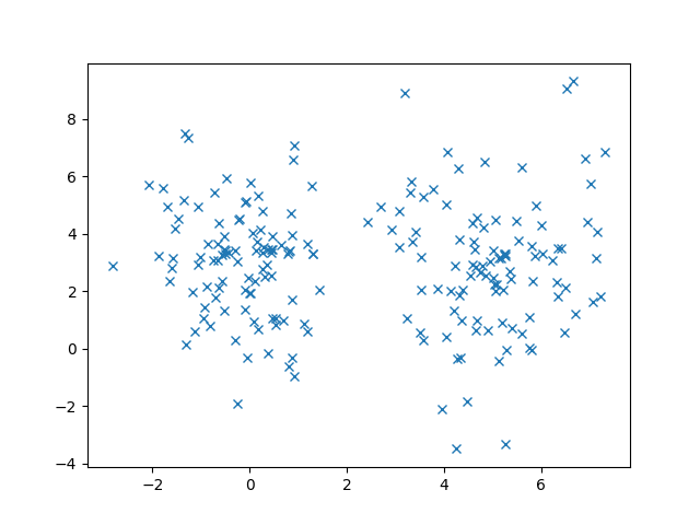
Given our dataset and $k$ , the number of clusters, we want to automatically find where to position the clusters. To make this example a bit more concrete, let’s consider a set of 200 data points.

The problem of clustering is to figure out where those $k$ clusters should be. From these data, we can figure out that there should be 2 clusters. Maybe the left cluster should be about $(-0.25, 2)$ and the right cluster should be about $(5.75, 2)$ . In fact, I’ve generated this data according to a specific algorithm, that I won’t reveal until later, so we can see how close our clustering algorithms get!

Choosing the Number of Clusters

One question that always comes up when discussing clustering algorithms is “how many clusters should I use?” From the clustering algorithm, we at least know that it should be strictly less than the number of data points! Naturally, there’s no right answer to this question, although there are many different heuristics that we could use to select this.

One such heuristic is simply to try many different values of $k$ and see which one works the best. In reality, there’s no one heuristic or algorithm that we can use to automatically determine the number of clusters each time. Sometimes, we just have to eyeball it! With 2D data, we can usually determine at least a good range of $k$ to try. In our above example, $k=2$ would be a good choice, but so might $k=4$ . We’re going to assume $k=2$ for the data that we’re dealing with.

K-Means Clustering

Let’s discuss k-means clustering. The algorithm itself is fairly intuitive so we’ll look at that first. Then, we’ll take a closer look at some nice properties of k-means clustering.

The k-means algorithm starts by randomly initializing the cluster centers. This random initialization step is very important! We’ll see the effects of poor initialization later. Then, we take each point in our dataset and assign it to the closest cluster center using the Euclidean distance from the cluster center to the point. At the end of this step, each point should be assigned to its closest cluster, i.e., there will never be an unassigned point (although there may be clusters with no assigned points). Then we update the position of the cluster by taking the mean of the points that are assigned to it. Then we assign each point to its closest cluster center again and repeat! How long do we repeat for? We repeat until convergence, and k-means will always converge (we’ll discuss the reason for this later).

Here is the k-means algorithm.

Randomly initialize cluster centers $\mu_1, \cdots, \mu_k}$
While not converged:
Assign each point to its closest cluster center
Update each $\mu_i$ to be the mean of all points assigned to that cluster

Now that we’ve seen the algorithm, let’s get to the code!

K-Means Clustering Code

First, download the ZIP file (link is at the beginning of this post). Inside, there is a file called data.pkl that has all of our data points. We can use Python’s pickle library to load data from this file and plot it using the following code snippet. We should see the same plot as above.

if __name__ == '__main__':
    with open('data.pkl', 'rb') as f:
        data = pickle.load(f)

    X = data['x']

    plt.plot(X[:,0], X[:,1], 'x')
    plt.show()

Remember that the k-means algorithm is an unsupervised algorithm so there are no ground-truth labels. Here, the matrix X holds all of our data, where each row is a data point and each column is a dimension, e.g., the dimensions of X should be 200×2 in our example above.

Now we can get started creating our class.

class KMeans(object):
    """Implementation of KMeans"""
    def __init__(self, k):
        self.k = k

The only parameter that we need is the number of clusters $k$ . Now we can start writing our function to initialize and move the cluster centers.

def fit(self, X):
    self.centers = X[np.random.randint(X.shape[0], size=self.k)]

    plt.plot(X[:,0], X[:,1], 'bx')
    plt.plot(self.centers[:,0], self.centers[:,1], 'ro')
    plt.show()

How do we randomly initialize our clusters? Let’s just randomly select $k$ points from our dataset to act as the initial cluster center. There are certainly more sophisticated ways of initializing the cluster centers, but this is the simplest and works well.

We will also be learning some new numpy tricks along the way. For example, inside of the brackets when we initialize the cluster centers, we’re actually giving numpy a list of indices. And this does exactly what you think! Numpy will give us a matrix back with the rows that correspond to those indices.

Now we can write the main loop.

while True:
    distances = np.sqrt(np.sum((X - self.centers[:, np.newaxis]) ** 2, axis=2))
    closestClusters = np.argmin(distances, axis=0)

First, we’re using an infinite loop, which would usually be a bit dangerous, but k-means has some nice properties about convergence that we’ll discuss later. The two lines after, we compute the Euclidean distance of each point to each cluster center and determine the index of the cluster. There is a lot going on in this first line, and we use another numpy trick.

The square root, sum, and square is just part of computing the Euclidean distance. The strange part of the code seems to be the following line.

X - self.centers[:, np.newaxis]

If we look at the resulting shape of the array, we see $2\times 200\times 2$ , but, in general, we would get $k\times n\times 2$ , where the shape is the number of cluster centers, number of data points, and the dimensionality of the data points, in that order. But wait, didn’t we only have 2 dimensions before? The extra dimension is from using np.newaxis. The extra dimension is only temporary since we need it to compute the Euclidean distance, the square root of the sum of the square of each input dimension (2 in our case).

With the last line above, we’re just selecting the index of the cluster that is closest to a given point. At the end of these lines of code, we know the index of the closest cluster for each point.

Next, we need to compute the new cluster centers by taking the mean of the set of data points that belongs to a cluster. We can do this efficiently in numpy in a single line of code.

newCenters = np.array([np.mean(X[closestClusters == c], axis=0) for c in range(self.k)])

In the innermost statement, X[closestClusters == c], we’re asking numpy to select all of the points who have $c$ as their closest cluster. Then we can take the mean point of that list of points.

Why don’t we update the cluster centers? Why do we create a new variable? This is because we need a way to break out of the infinite loop. When k-means converges, our cluster centers have settled and do not move! We can write code to check for this and break out of the loop if the new cluster centers haven’t changed.

if np.all(self.centers - newCenters < 1e-5):
    break
self.centers = newCenters

Since we’re dealing with floating-point numbers, we actually have a small margin of $10^{-5}$ . If we have moved more than that, then we update the cluster centers.

Here’s the entire code for the main k-means function.

def fit(self, X):
    self.centers = X[np.random.randint(X.shape[0], size=self.k)]


    plt.plot(X[:,0], X[:,1], 'bx')
    plt.plot(self.centers[:,0], self.centers[:,1], 'ro')
    plt.show()

    while True:
        distances = np.sqrt(np.sum((X - self.centers[:, np.newaxis]) ** 2, axis=2))
        closestClusters = np.argmin(distances, axis=0)

        newCenters = np.array([np.mean(X[closestClusters == c], axis=0) for c in range(self.k)])
        if np.all(self.centers - newCenters < 1e-5):
            break
        self.centers = newCenters

    plt.plot(X[:,0], X[:,1], 'bx')
    plt.plot(self.centers[:,0], self.centers[:,1], 'ro')
    plt.show()

There’s also code that displays the initial and final cluster positions.

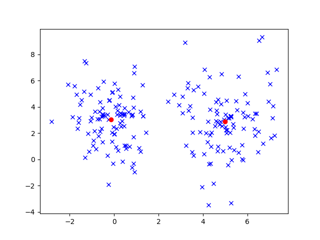
This figure shows an example of what we might expect to see with K-Means. In fact, the final cluster positions are very close to the right answer! I generated this data using two multivariate Gaussian distributions centered at $(0, 3)$ and $(5, 3)$ .

Due to random initialization, it might be the case that your cluster centers converged to a different location. Usually, the cluster centers will be pretty close to the true centers. (Obviously, when dealing with real-world data, we can’t possibly know where the true centers are!) But there are some instances where poor initialization can lead to bad results.

Poor Initialization of Cluster Centers

Good initialization of the cluster centers is critical to good results! Consider the following figure.

This is an example of poor initialization! The cluster centers are not near the true values at all. (To generate this, I manually initialized the cluster centers to bad values.) This is certainly a possibility when using clustering algorithms that randomly initialize data.

How can we combat this? A simple, but effective, technique to prevent this to run the k-means algorithm for multiple trials and take the average of the final cluster centers. This way, if we have poor initialization for a few trials, they won’t affect our final results much. There are more sophisticated ways than taking an average, e.g., build a distribution over the cluster centers from all trials and get rid of any final cluster positions that are some distance away from the mean.

K-Means Convergence

Now that we’ve discussed the algorithm, there’s still a question we haven’t answered yet: How do we know the k-means algorithm will converge? To answer this question, we have to look at its cost function.

$J = \displaystyle\sum_{j=1}^{k}\sum_{i\in C_j} || x_i - \mu_j ||^2$

At a high level, the cost is measured by computing the sum of all points from their assigned cluster for all clusters. The cost function is at a minimum when, for each cluster, it is positioned so that the cluster center is a minimal distance from each point assigned to it.

The inner sum is over a particular cluster $j$ . It takes the sum of the distance from all points that belong to cluster $j$ to the cluster center of cluster $j$ . Then the outer sum simply sums over all clusters.

We won’t really prove this, but I’ll provide an intuitive understanding as to why k-means converges and doesn’t keep iterating to infinity. The idea hinges on the fact that, at each step of the loop, the cost value at the new cluster center must be less than or equal to than the previous cluster center location. In other words, the cost is monotonically decreasing since we’re updating the centers based only on the data. Notice that the cluster centers update does not depend on the previous location! (There is a formal convergence proof that proves k-means converges in a finite number of steps, but I’ve skipped over that since the intuition is more useful than the proof.) Hence, k-means will keep iterating until the new cost value is the same as the old one. We have a conditional check for this in our code, and that’s where we break out of the loop. There may be cases where k-means takes a long time; in those cases, we could replace the infinite while loop with a finite loop that iterates until the maximum number of allowable iterations is met.

One important thing to note is that there’s no guarantee that it will converge to the right answer or even an answer that makes sense! (Theoretically, computing the global minimum, i.e., the optimal answer, is an NP-hard problem.) The only guarantee is that k-means will stop, i.e., the cluster centers will stop moving, in a finite amount of steps.

To summarize, we discussed the most popular clustering algorithm: k-means clustering. This is an intuitive algorithm that, given the number of clusters, can automatically find out where the clusters should be. First, we randomly initialize the cluster centers. Then we assign each point to its closest cluster and update the cluster center to be the mean of the set of all points assigned to it. After we perform this update, we simply re-assign each point and repeat until the algorithm converges. We discussed some critical aspects of this algorithm such as initialization and convergence. In addition, we learned some numpy tricks along the way.

In practice, the k-means algorithm is very popular and the first-used algorithm when given a clustering task.